- Beating the lower bound with counting sort

Содержание
- 2. A Lower Bound for Sorting Rules for sorting. The lower bound on comparison sorting. Beating the
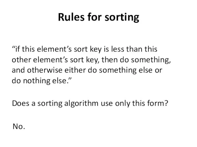
- 3. “if this element’s sort key is less than this other element’s sort key, then do something,
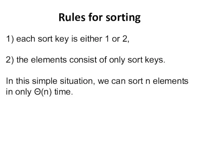
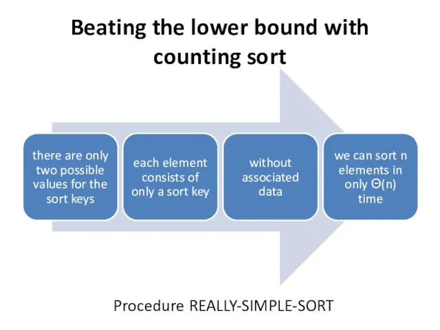
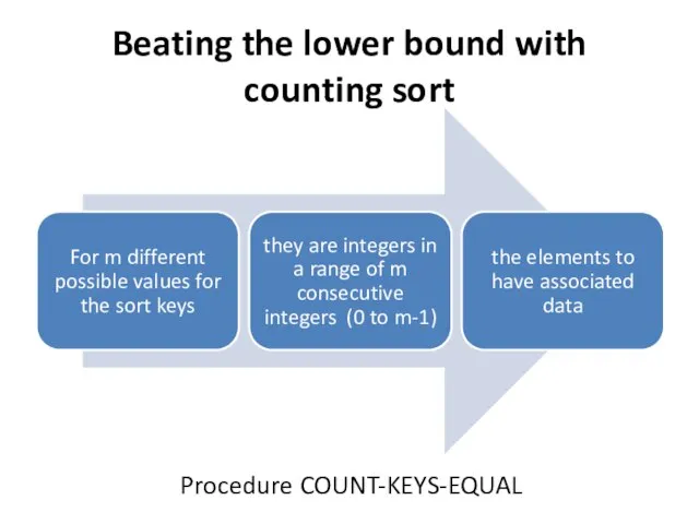
- 4. 1) each sort key is either 1 or 2, 2) the elements consist of only sort
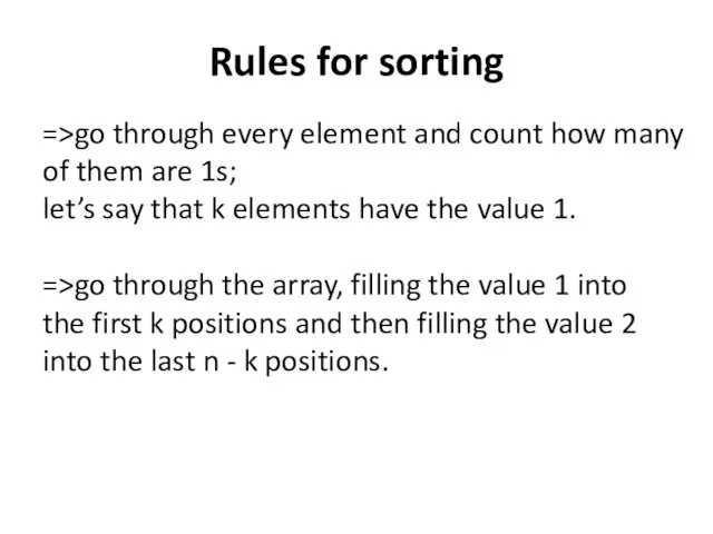
- 5. =>go through every element and count how many of them are 1s; let’s say that k
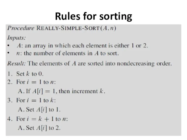
- 6. Rules for sorting
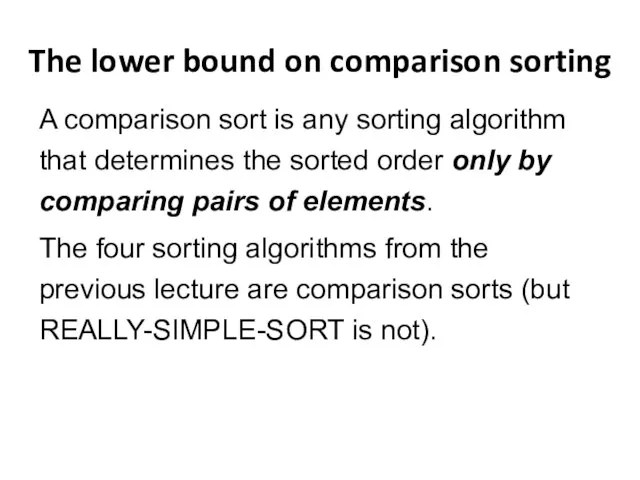
- 7. The lower bound on comparison sorting A comparison sort is any sorting algorithm that determines the
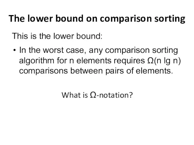
- 8. The lower bound on comparison sorting This is the lower bound: In the worst case, any
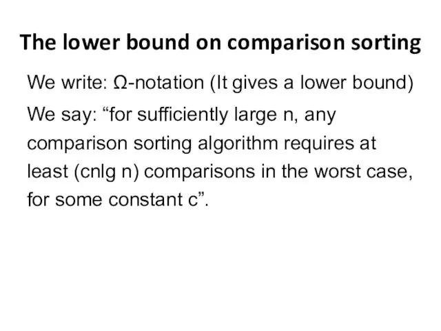
- 9. The lower bound on comparison sorting We write: Ω-notation (It gives a lower bound) We say:
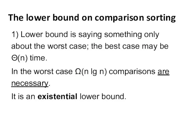
- 10. The lower bound on comparison sorting 1) Lower bound is saying something only about the worst
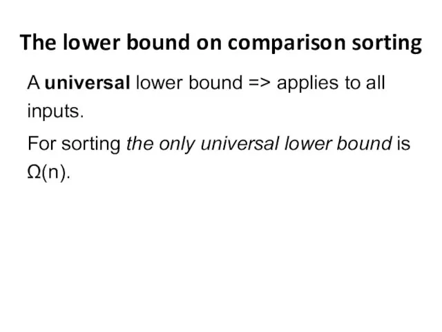
- 11. The lower bound on comparison sorting A universal lower bound => applies to all inputs. For
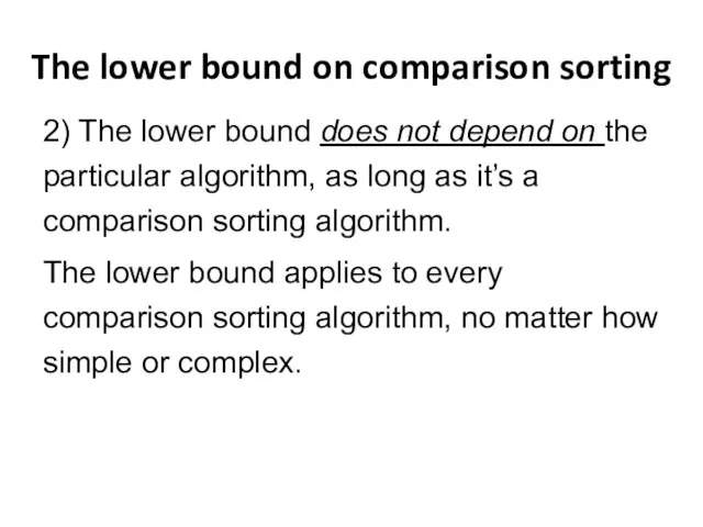
- 12. The lower bound on comparison sorting 2) The lower bound does not depend on the particular
- 13. Beating the lower bound with counting sort Procedure REALLY-SIMPLE-SORT
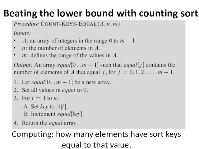
- 14. Beating the lower bound with counting sort Procedure COUNT-KEYS-EQUAL
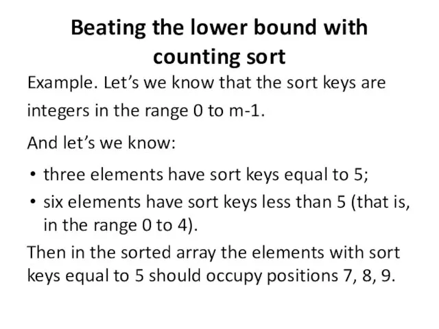
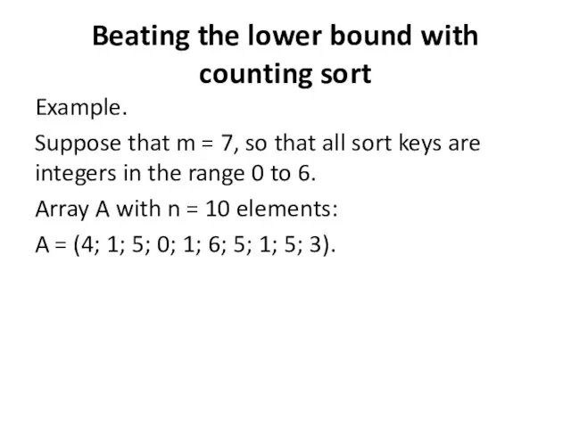
- 15. Beating the lower bound with counting sort Example. Let’s we know that the sort keys are
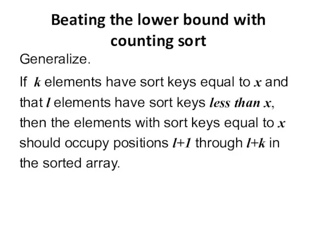
- 16. Beating the lower bound with counting sort Generalize. If k elements have sort keys equal to
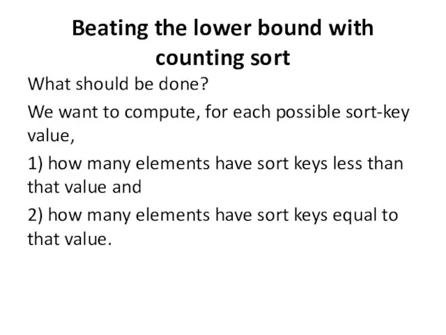
- 17. Beating the lower bound with counting sort What should be done? We want to compute, for
- 18. Beating the lower bound with counting sort Computing: how many elements have sort keys equal to
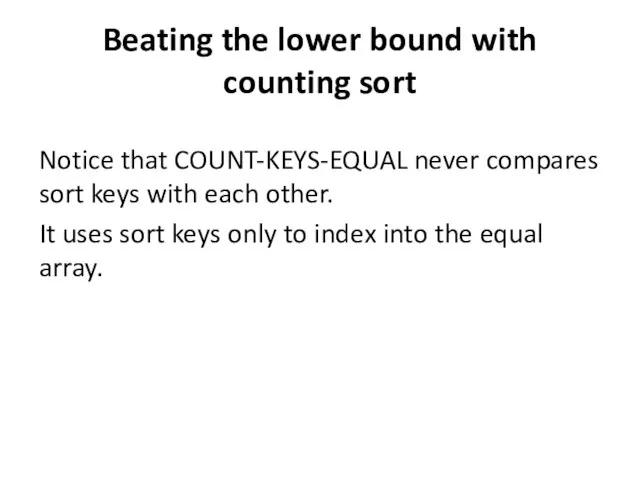
- 19. Beating the lower bound with counting sort Notice that COUNT-KEYS-EQUAL never compares sort keys with each
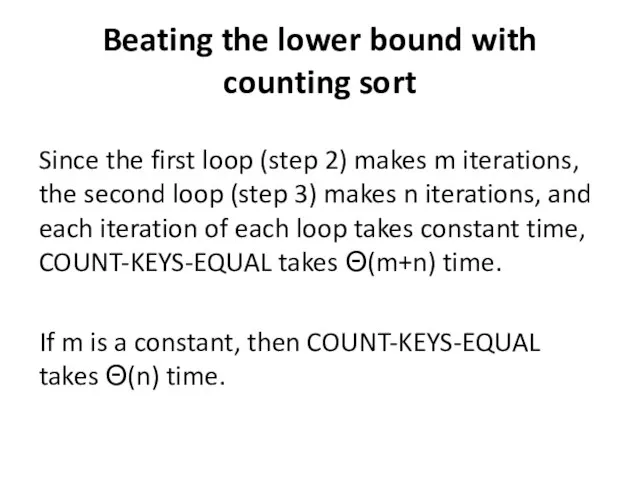
- 20. Beating the lower bound with counting sort Since the first loop (step 2) makes m iterations,
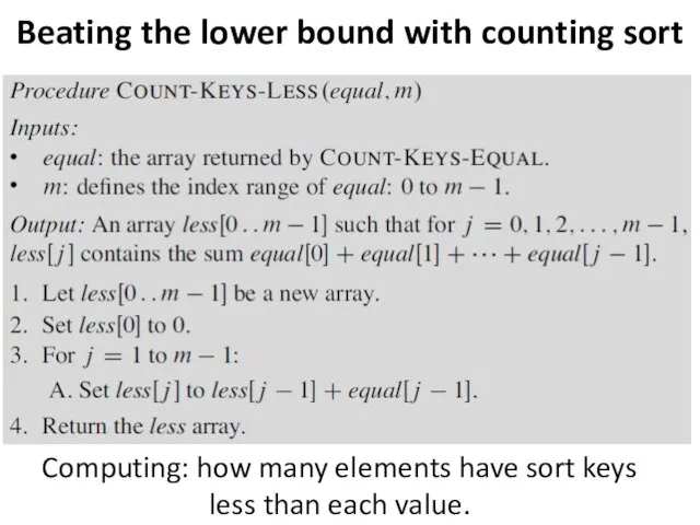
- 21. Beating the lower bound with counting sort Computing: how many elements have sort keys less than
- 22. Beating the lower bound with counting sort Example. Suppose that m = 7, so that all
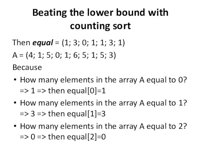
- 23. Beating the lower bound with counting sort Then equal = (1; 3; 0; 1; 1; 3;
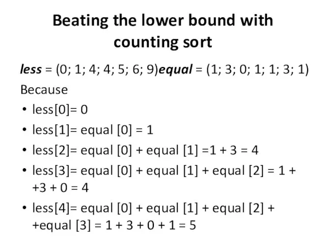
- 24. Beating the lower bound with counting sort less = (0; 1; 4; 4; 5; 6; 9)equal
- 26. Example.
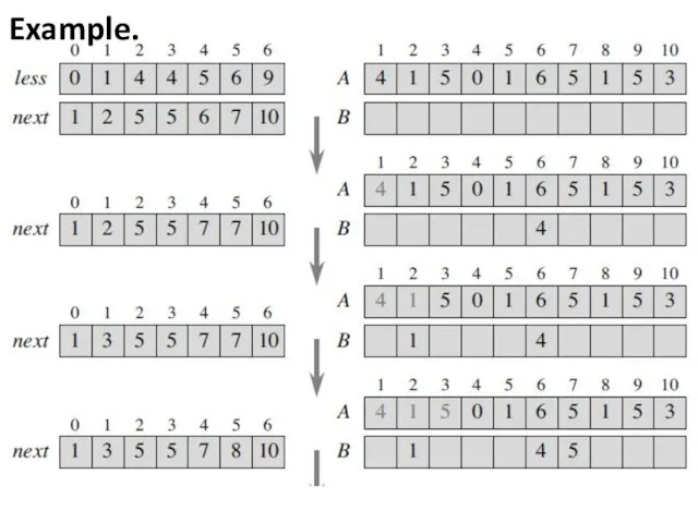
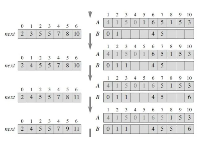
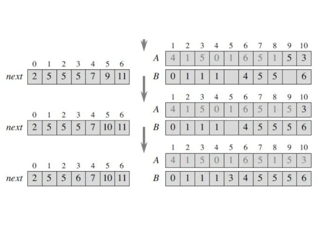
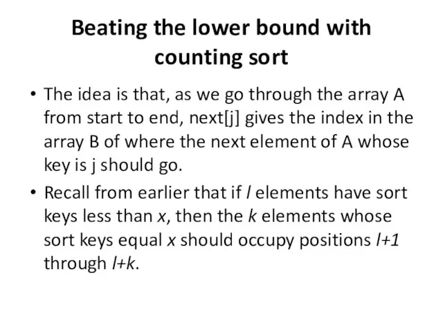
- 30. Beating the lower bound with counting sort The idea is that, as we go through the
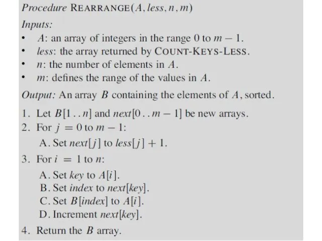
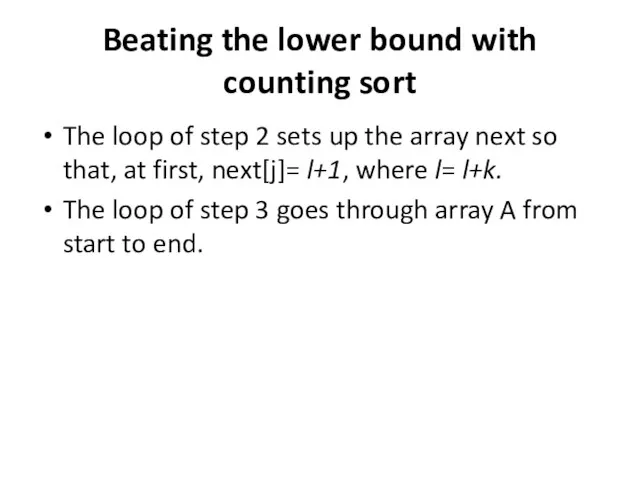
- 31. Beating the lower bound with counting sort The loop of step 2 sets up the array
- 32. Beating the lower bound with counting sort For each element A[i], step 3A stores A[i] into
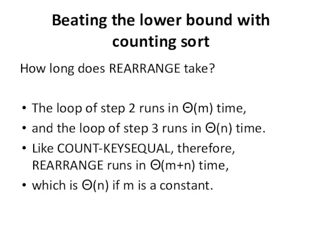
- 33. Beating the lower bound with counting sort How long does REARRANGE take? The loop of step
- 34. Beating the lower bound with counting sort Counting sort
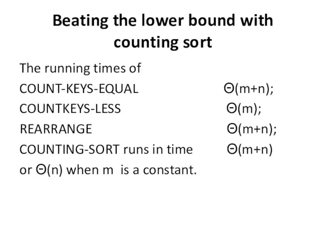
- 35. Beating the lower bound with counting sort The running times of COUNT-KEYS-EQUAL Θ(m+n); COUNTKEYS-LESS Θ(m); REARRANGE
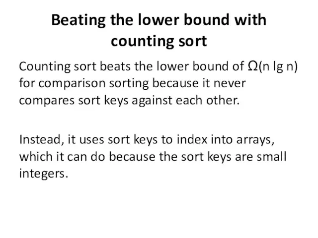
- 36. Beating the lower bound with counting sort Counting sort beats the lower bound of Ω(n lg
- 37. Beating the lower bound with counting sort If the sort keys were real numbers with fractional
- 38. Beating the lower bound with counting sort The running time is Θ(n) if m is a
- 39. Beating the lower bound with counting sort Sorting exams by grade. The grades range from 0
- 40. Beating the lower bound with counting sort Counting sort has another important property: it is stable.
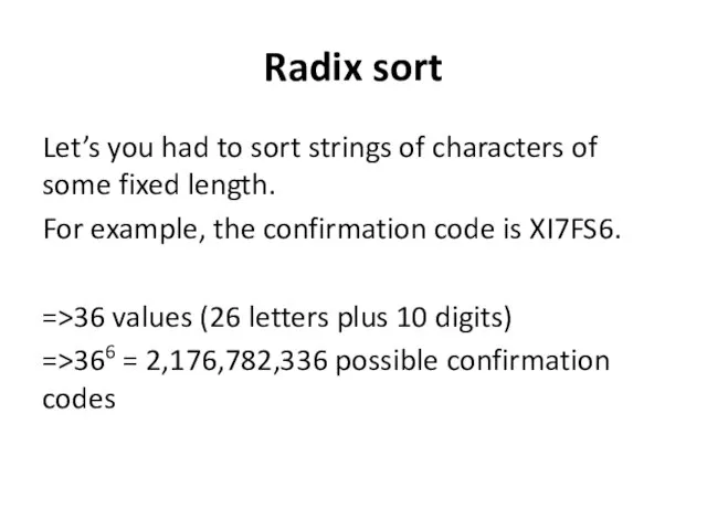
- 41. Radix sort Let’s you had to sort strings of characters of some fixed length. For example,
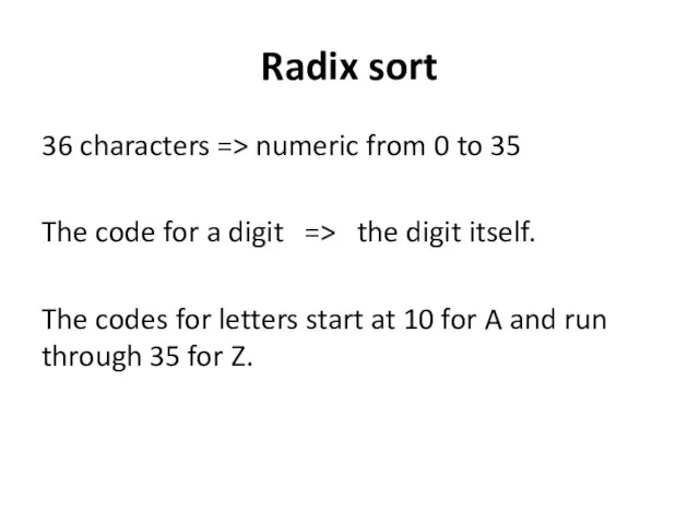
- 42. Radix sort 36 characters => numeric from 0 to 35 The code for a digit =>
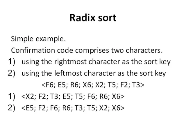
- 43. Radix sort Simple example. Confirmation code comprises two characters. using the rightmost character as the sort
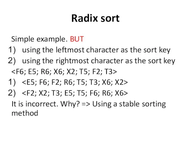
- 44. Radix sort Simple example. BUT using the leftmost character as the sort key using the rightmost
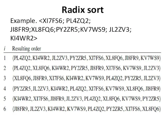
- 45. Radix sort Example.
- 47. Скачать презентацию
Слайд 3“if this element’s sort key is less than this
other element’s sort
“if this element’s sort key is less than this
other element’s sort
Слайд 41) each sort key is either 1 or 2,
2) the elements
1) each sort key is either 1 or 2,
2) the elements
Слайд 5=>go through every element and count how many
of them are 1s;
=>go through every element and count how many
of them are 1s;
Слайд 6Rules for sorting
Rules for sorting
Слайд 7The lower bound on comparison sorting
A comparison sort is any sorting algorithm
The lower bound on comparison sorting
A comparison sort is any sorting algorithm
Слайд 8The lower bound on comparison sorting
This is the lower bound:
In the
The lower bound on comparison sorting
This is the lower bound:
In the
Слайд 9The lower bound on comparison sorting
We write: Ω-notation (It gives a lower
The lower bound on comparison sorting
We write: Ω-notation (It gives a lower
Слайд 10The lower bound on comparison sorting
1) Lower bound is saying something only
The lower bound on comparison sorting
1) Lower bound is saying something only
Слайд 11The lower bound on comparison sorting
A universal lower bound => applies to
The lower bound on comparison sorting
A universal lower bound => applies to
Слайд 12The lower bound on comparison sorting
2) The lower bound does not depend
The lower bound on comparison sorting
2) The lower bound does not depend
Слайд 13Beating the lower bound with
counting sort
Procedure REALLY-SIMPLE-SORT
Beating the lower bound with
counting sort
Procedure REALLY-SIMPLE-SORT
Слайд 14Beating the lower bound with
counting sort
Procedure COUNT-KEYS-EQUAL
Beating the lower bound with
counting sort
Procedure COUNT-KEYS-EQUAL
Слайд 15Beating the lower bound with
counting sort
Example. Let’s we know that the
Beating the lower bound with
counting sort
Example. Let’s we know that the
Слайд 16Beating the lower bound with
counting sort
Generalize.
If k elements have sort keys
Beating the lower bound with
counting sort
Generalize.
If k elements have sort keys
Слайд 17Beating the lower bound with
counting sort
What should be done?
We want
Beating the lower bound with
counting sort
What should be done?
We want
Слайд 18Beating the lower bound with counting sort
Computing: how many elements have sort
Beating the lower bound with counting sort
Computing: how many elements have sort
Слайд 19Beating the lower bound with
counting sort
Notice that COUNT-KEYS-EQUAL never compares sort
Beating the lower bound with
counting sort
Notice that COUNT-KEYS-EQUAL never compares sort
Слайд 20Beating the lower bound with
counting sort
Since the first loop (step 2)
Beating the lower bound with
counting sort
Since the first loop (step 2)
Слайд 21Beating the lower bound with counting sort
Computing: how many elements have sort
Beating the lower bound with counting sort
Computing: how many elements have sort
Слайд 22Beating the lower bound with
counting sort
Example.
Suppose that m = 7, so
Beating the lower bound with
counting sort
Example.
Suppose that m = 7, so
Слайд 23Beating the lower bound with
counting sort
Then equal = (1; 3; 0;
Beating the lower bound with
counting sort
Then equal = (1; 3; 0;
Слайд 24Beating the lower bound with
counting sort
less = (0; 1; 4; 4;
Beating the lower bound with
counting sort
less = (0; 1; 4; 4;
Слайд 26Example.
Example.

Слайд 30Beating the lower bound with
counting sort
The idea is that, as we
Beating the lower bound with
counting sort
The idea is that, as we
Слайд 31Beating the lower bound with
counting sort
The loop of step 2 sets
Beating the lower bound with
counting sort
The loop of step 2 sets
Слайд 32Beating the lower bound with
counting sort
For each element A[i], step 3A
Beating the lower bound with
counting sort
For each element A[i], step 3A
![Beating the lower bound with counting sort For each element A[i], step](/_ipx/f_webp&q_80&fit_contain&s_1440x1080/imagesDir/jpg/851702/slide-31.jpg)
Слайд 33Beating the lower bound with
counting sort
How long does REARRANGE take?
The loop
Beating the lower bound with
counting sort
How long does REARRANGE take?
The loop
Слайд 34Beating the lower bound with
counting sort
Counting sort
Beating the lower bound with
counting sort
Counting sort

Слайд 35Beating the lower bound with
counting sort
The running times of
COUNT-KEYS-EQUAL Θ(m+n);
COUNTKEYS-LESS
Beating the lower bound with
counting sort
The running times of
COUNT-KEYS-EQUAL Θ(m+n);
COUNTKEYS-LESS
Слайд 36Beating the lower bound with
counting sort
Counting sort beats the lower bound
Beating the lower bound with
counting sort
Counting sort beats the lower bound
Слайд 37Beating the lower bound with
counting sort
If the sort keys were real
Beating the lower bound with
counting sort
If the sort keys were real
Слайд 38Beating the lower bound with
counting sort
The running time is Θ(n) if
Beating the lower bound with
counting sort
The running time is Θ(n) if
Слайд 39Beating the lower bound with
counting sort
Sorting exams by grade.
The grades
Beating the lower bound with
counting sort
Sorting exams by grade.
The grades
Слайд 40Beating the lower bound with
counting sort
Counting sort has another important property:
Beating the lower bound with
counting sort
Counting sort has another important property:
Слайд 41Radix sort
Let’s you had to sort strings of characters of some fixed
Radix sort
Let’s you had to sort strings of characters of some fixed
Слайд 42Radix sort
36 characters => numeric from 0 to 35
The code for a
Radix sort
36 characters => numeric from 0 to 35
The code for a
Слайд 43Radix sort
Simple example.
Confirmation code comprises two characters.
using the rightmost character as the
Radix sort
Simple example.
Confirmation code comprises two characters.
using the rightmost character as the
Слайд 44Radix sort
Simple example. BUT
using the leftmost character as the sort key
using the
Radix sort
Simple example. BUT
using the leftmost character as the sort key
using the
Слайд 45Radix sort
Example.
Radix sort
Example.
 Введение Последние годы развития GSM-связи на рынке показали существенный рост объема передаваемых данных. В этом росте есть и засл
 Особенности средневековой моды
 Конфликты в общении, формы и способы их разрешения
 Рельсовая пушка
 Презентация на тему Добро и зло
 Современные актеры театра и кино
 Презентация на тему Изучение реакции среды в зависимости от типа гидролиза соли
 Презентация на тему ПИЗАНСКАЯ БАШНЯ
  Christmas traditions
 Регулировщик РЭАиП
 Уголок России - отчий дом
 Управление проектами по разработке ПО в корпорациях Руслан Мартимов. Менеджер проектов разработки ПО. Корпорация General Satellite.
 Внешнеторговый контракт. Базисные условия поставок
 Опыт развития риэлторской компании в Северо-Западном регионе
 Основные сведения о металлорежущих станках
 Муниципальное автономное дошкольное образовательное учреждение «Детский сад № 40 «Алёнушка» общеразвивающего вида»
 Презентация на тему Анализ поэмы Гоголя Мертвые души
  Управление экспертной деятельностью. Prof IT
 «Административная реформа: цели, задачи, методы реализации»
 20140107_zapadno-sibirskaya
 Агентство экономической диверсификации западных провинций Канады Western Economic Diversification Canada Автор доклада: Даг Мейли, Заместитель ми
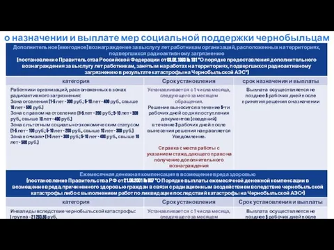 Назначении и выплате мер социальной поддержки чернобыльцам
 Синтетическая природа фильма и монтаж
 Презентация на тему Коррекционная группа
 История возникновения Масленицы
 Обучение химии
 Сетевые программы повышения квалификации
 Романтизм в живописи