- Perfect Conpetition and the supply Curve

Содержание
- 2. What a perfectly competitive market is and the characteristics of a perfectly competitive industry How a
- 3. Perfect Competition A price-taking producer is a producer whose actions have no effect on the market
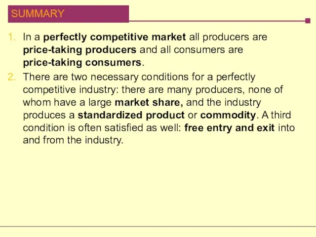
- 4. Two Necessary Conditions for Perfect Competition For an industry to be perfectly competitive, it must contain
- 5. Free Entry and Exit There is free entry and exit into and from an industry when
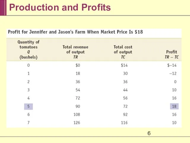
- 6. Production and Profits
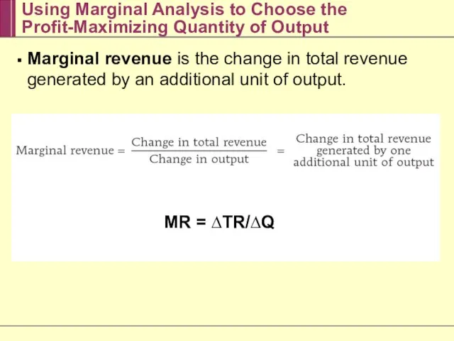
- 7. Using Marginal Analysis to Choose the Profit-Maximizing Quantity of Output Marginal revenue is the change in
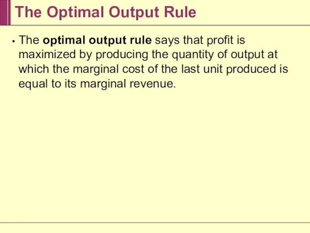
- 8. The Optimal Output Rule The optimal output rule says that profit is maximized by producing the
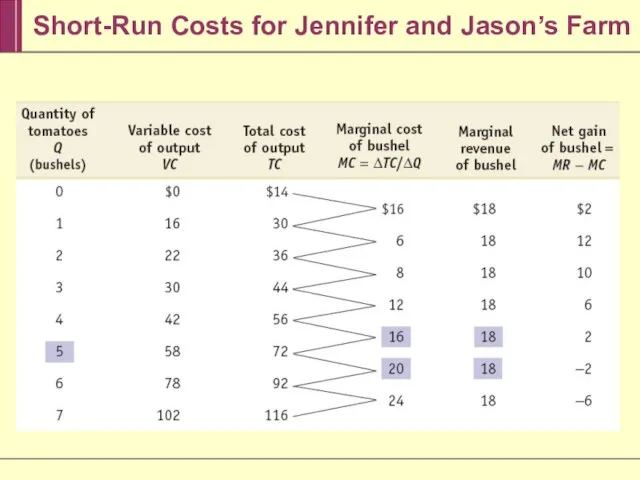
- 9. Short-Run Costs for Jennifer and Jason’s Farm
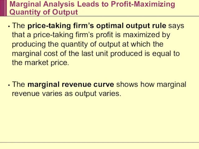
- 10. Marginal Analysis Leads to Profit-Maximizing Quantity of Output The price-taking firm’s optimal output rule says that
- 11. The Price-Taking Firm’s Profit-Maximizing Quantity of Output 7 6 5 4 3 2 1 0 $24
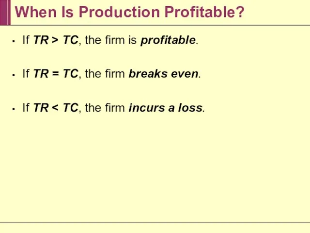
- 12. When Is Production Profitable? If TR > TC, the firm is profitable. If TR = TC,
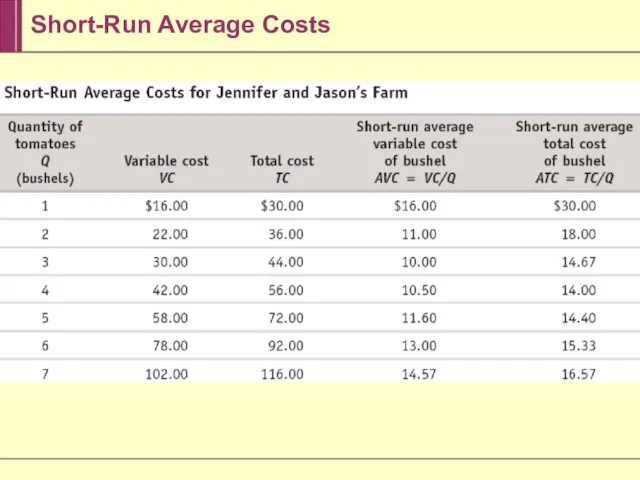
- 13. Short-Run Average Costs
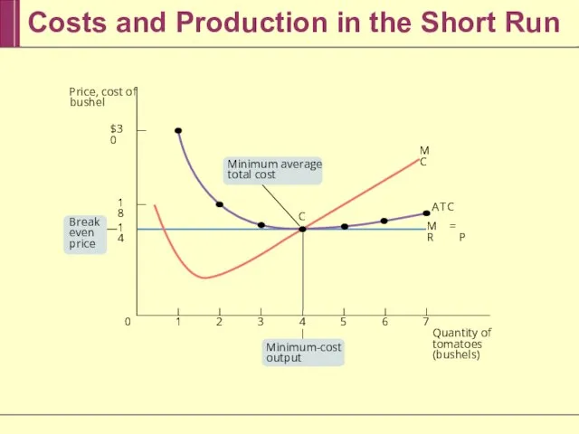
- 14. Costs and Production in the Short Run 7 6 5 4 3 2 1 0 $30
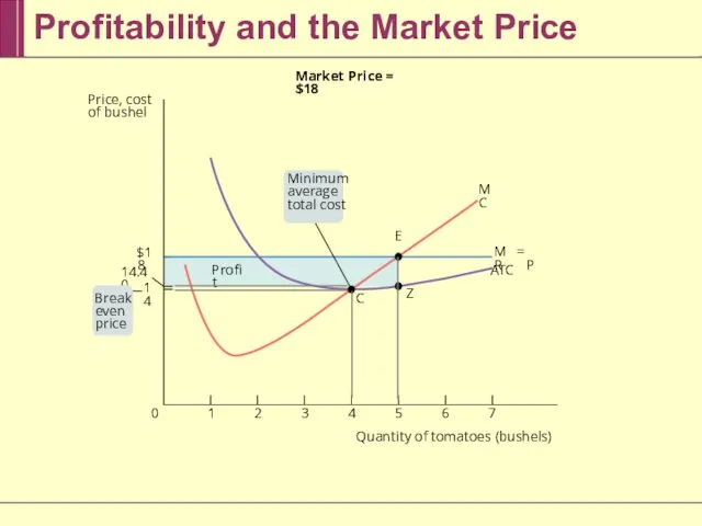
- 15. Profitability and the Market Price 7 6 5 4 3 2 1 0 MC Profit A
- 16. Profitability and the Market Price 7 6 5 4 3 2 1 0 MC Loss A
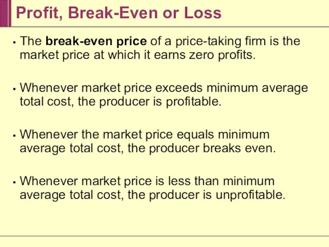
- 17. Profit, Break-Even or Loss The break-even price of a price-taking firm is the market price at
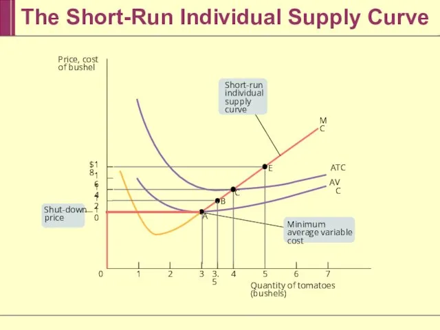
- 18. The Short-Run Individual Supply Curve 7 6 5 4 3 3.5 2 1 0 $18 16
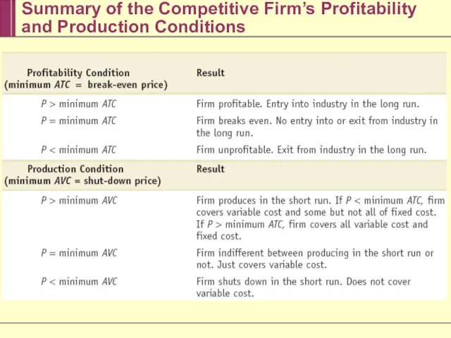
- 19. Summary of the Competitive Firm’s Profitability and Production Conditions
- 20. Industry Supply Curve The industry supply curve shows the relationship between the price of a good
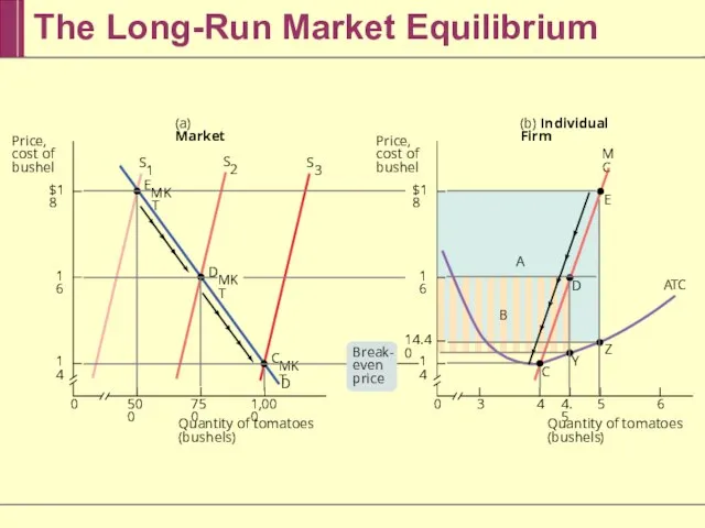
- 21. The Long-Run Industry Supply Curve A market is in long-run market equilibrium when the quantity supplied
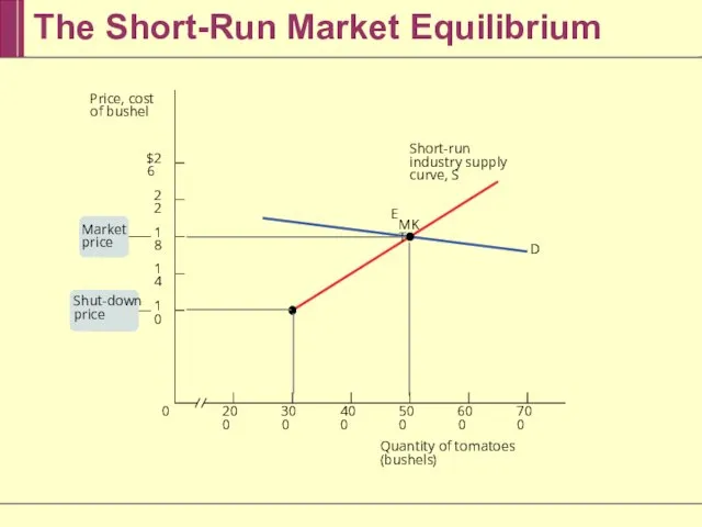
- 22. The Short-Run Market Equilibrium 700 600 500 400 300 200 0 $26 22 18 14 10
- 23. The Long-Run Market Equilibrium Quantity of tomatoes (bushels) 6 5 4 4.5 3 0 $18 16
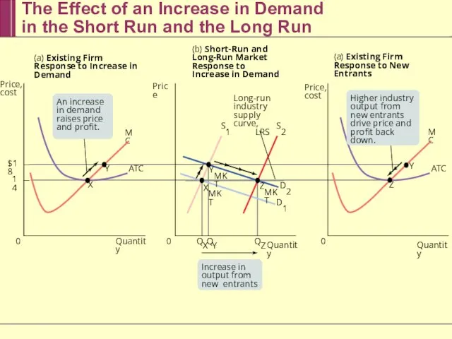
- 24. The Effect of an Increase in Demand in the Short Run and the Long Run MC
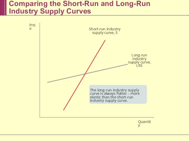
- 25. Comparing the Short-Run and Long-Run Industry Supply Curves The long-run industry supply curve is always flatter
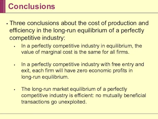
- 26. Conclusions Three conclusions about the cost of production and efficiency in the long-run equilibrium of a
- 27. In a perfectly competitive market all producers are price-taking producers and all consumers are price-taking consumers.
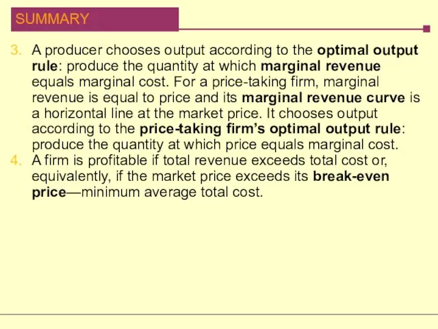
- 28. A producer chooses output according to the optimal output rule: produce the quantity at which marginal
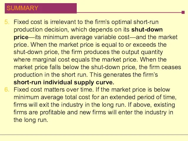
- 29. Fixed cost is irrelevant to the firm’s optimal short-run production decision, which depends on its shut-down
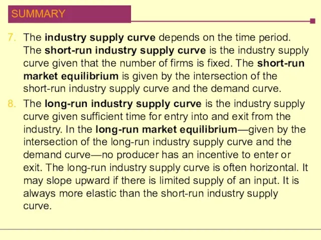
- 30. The industry supply curve depends on the time period. The short-run industry supply curve is the
- 32. Скачать презентацию
Слайд 3Perfect Competition
A price-taking producer is a producer whose actions have no effect
Perfect Competition
A price-taking producer is a producer whose actions have no effect
Слайд 4Two Necessary Conditions for Perfect Competition
For an industry to be perfectly competitive,
Two Necessary Conditions for Perfect Competition
For an industry to be perfectly competitive,
Слайд 5Free Entry and Exit
There is free entry and exit into and from
Free Entry and Exit
There is free entry and exit into and from
Слайд 6Production and Profits
Production and Profits
Слайд 7Using Marginal Analysis to Choose the Profit-Maximizing Quantity of Output
Marginal revenue is
Using Marginal Analysis to Choose the Profit-Maximizing Quantity of Output
Marginal revenue is
Слайд 8The Optimal Output Rule
The optimal output rule says that profit is maximized
The Optimal Output Rule
The optimal output rule says that profit is maximized
Слайд 9Short-Run Costs for Jennifer and Jason’s Farm
Short-Run Costs for Jennifer and Jason’s Farm
Слайд 10Marginal Analysis Leads to Profit-Maximizing Quantity of Output
The price-taking firm’s optimal output
Marginal Analysis Leads to Profit-Maximizing Quantity of Output
The price-taking firm’s optimal output
Слайд 11The Price-Taking Firm’s Profit-Maximizing Quantity of Output
7
6
5
4
3
2
1
0
$24
20
18
16
12
8
6
Price, cost of bushel
Quantity of tomatoes
The Price-Taking Firm’s Profit-Maximizing Quantity of Output
7
6
5
4
3
2
1
0
$24
20
18
16
12
8
6
Price, cost of bushel
Quantity of tomatoes

Слайд 12When Is Production Profitable?
If TR > TC, the firm is profitable.
If TR
When Is Production Profitable?
If TR > TC, the firm is profitable.
If TR
Слайд 13Short-Run Average Costs
Short-Run Average Costs
Слайд 14Costs and Production in the Short Run
7
6
5
4
3
2
1
0
$30
18
14
MC
A
T
C
MR
=
P
C
Break even price
Minimum-cost output
Price,
Costs and Production in the Short Run
7
6
5
4
3
2
1
0
$30
18
14
MC
A
T
C
MR
=
P
C
Break even price
Minimum-cost output
Price,
Слайд 15Profitability and the Market Price
7
6
5
4
3
2
1
0
MC
Profit
A
T
C
MR
=
P
C
Z
E
Market Price = $18
14
14.40
$18
Price, cost of
Profitability and the Market Price
7
6
5
4
3
2
1
0
MC
Profit
A
T
C
MR
=
P
C
Z
E
Market Price = $18
14
14.40
$18
Price, cost of
Слайд 16Profitability and the Market Price
7
6
5
4
3
2
1
0
MC
Loss
A
T
C
MR
=
P
C
A
Y
Market Price = $10
14
10
$14.67
Price, cost of
Profitability and the Market Price
7
6
5
4
3
2
1
0
MC
Loss
A
T
C
MR
=
P
C
A
Y
Market Price = $10
14
10
$14.67
Price, cost of
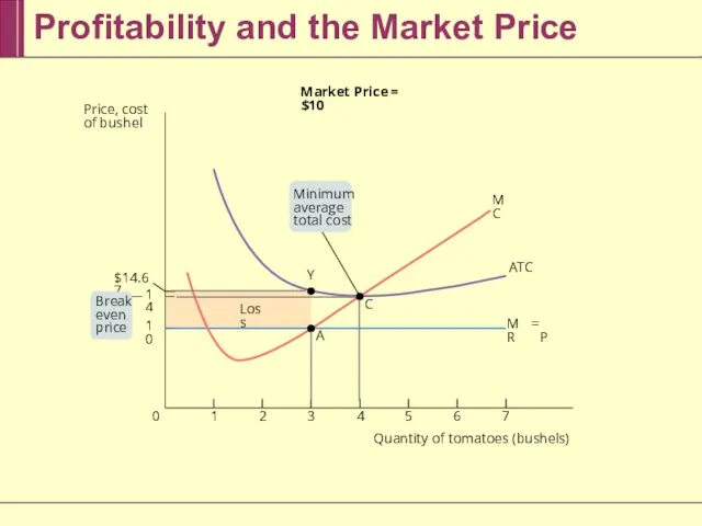
Слайд 17Profit, Break-Even or Loss
The break-even price of a price-taking firm is the
Profit, Break-Even or Loss
The break-even price of a price-taking firm is the
Слайд 18The Short-Run Individual Supply Curve
7
6
5
4
3
3.5
2
1
0
$18
16
14
12
10
MC
A
T
C
A
VC
C
B
A
E
Minimum average variable cost
Short-run individual supply curve
Shut-down price
Price,
The Short-Run Individual Supply Curve
7
6
5
4
3
3.5
2
1
0
$18
16
14
12
10
MC
A
T
C
A
VC
C
B
A
E
Minimum average variable cost
Short-run individual supply curve
Shut-down price
Price,
Слайд 19Summary of the Competitive Firm’s Profitability and Production Conditions
Summary of the Competitive Firm’s Profitability and Production Conditions
Слайд 20Industry Supply Curve
The industry supply curve shows the relationship between the price
Industry Supply Curve
The industry supply curve shows the relationship between the price
Слайд 21The Long-Run Industry Supply Curve
A market is in long-run market equilibrium when
The Long-Run Industry Supply Curve
A market is in long-run market equilibrium when
Слайд 22The Short-Run Market Equilibrium
700
600
500
400
300
200
0
$26
22
18
14
10
D
Short-run industry supply curve, S
E
MKT
Shut-down price
Price, cost of bushel
Quantity
The Short-Run Market Equilibrium
700
600
500
400
300
200
0
$26
22
18
14
10
D
Short-run industry supply curve, S
E
MKT
Shut-down price
Price, cost of bushel
Quantity
Слайд 23The Long-Run Market Equilibrium
Quantity of tomatoes (bushels)
6
5
4
4.5
3
0
$18
16
14
1,000
750
500
0
$18
16
14
D
E
C
D
Y
Z
MC
A
T
C
A
B
(a) Market
(b) Individual Firm
14.40
E
D
C
MKT
S
1
S
3
S
2
Price, cost of
The Long-Run Market Equilibrium
Quantity of tomatoes (bushels)
6
5
4
4.5
3
0
$18
16
14
1,000
750
500
0
$18
16
14
D
E
C
D
Y
Z
MC
A
T
C
A
B
(a) Market
(b) Individual Firm
14.40
E
D
C
MKT
S
1
S
3
S
2
Price, cost of
Слайд 24The Effect of an Increase in Demand
in the Short Run and the
The Effect of an Increase in Demand in the Short Run and the
Слайд 25Comparing the Short-Run and Long-Run
Industry Supply Curves
The long-run industry supply curve
Comparing the Short-Run and Long-Run
Industry Supply Curves
The long-run industry supply curve
Слайд 26Conclusions
Three conclusions about the cost of production and efficiency in the long-run
Conclusions
Three conclusions about the cost of production and efficiency in the long-run
Слайд 27In a perfectly competitive market all producers are price-taking producers and all
In a perfectly competitive market all producers are price-taking producers and all
Слайд 28A producer chooses output according to the optimal output rule: produce the
A producer chooses output according to the optimal output rule: produce the
Слайд 29Fixed cost is irrelevant to the firm’s optimal short-run production decision, which
Fixed cost is irrelevant to the firm’s optimal short-run production decision, which
Слайд 30The industry supply curve depends on the time period. The short-run industry
The industry supply curve depends on the time period. The short-run industry
 Итоговая аттестация пилотного класса в рамках реализации ФГОС НОО
 Достоевский Ф.М
 Вредные привычки у детей. Консультация для родителей
 ТКС
ТКС Измерение удельной теплоемкости твердого тела
 «Деревня…
 Церкви Ленинграда в годы Советской власти
 Условия и механизмы функционирования рынка информационных услуг и продуктов
 Презентация на тему Жизнь и творчество И.К. Айвазовского
 Это – Кинематограф!
 Классификация видов групп однородной продукции и их характеристики
 Погрузочно-доставочная машина LH514L
 Удивительная
 Лекция 3 Общение как социально-психологический механизм
 Организация и техническое оснащение работ по приготовлению, хранению, подготовке к реализации горячих соусов
 Кривая Филлипса: выбор между безработицей и инфляцией
 ГИА по русскому языку
 Тема 5 (Форми дежави)
 собственность эк 11
 Найбільші біржі світу. 9 клас
 АЙСБЕРГ
 Система оценки эффективности исполнителя и удовлетворенности клиента качеством сервиса по выполненным заявкам
 Product Placement
 Мои жизненные ценности
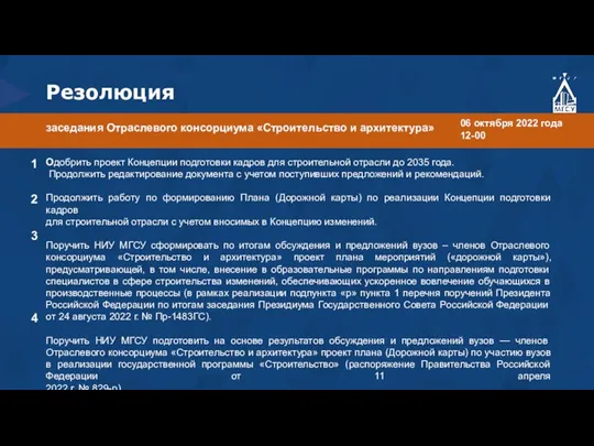 2022-10-6 Резолюция № 1 (1)
 Классические технологии хитрости на экзамене
 Презентация на тему Освоение культурного наследия Многоканальная модель освоения культурного наследия
  Malsharuashylyq