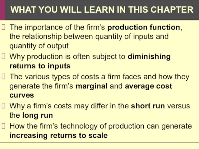
- Behind the supply Inputs and costs

Содержание
- 2. The importance of the firm’s production function, the relationship between quantity of inputs and quantity of
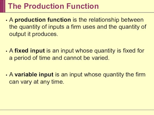
- 3. The Production Function A production function is the relationship between the quantity of inputs a firm
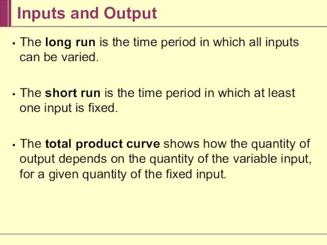
- 4. Inputs and Output The long run is the time period in which all inputs can be
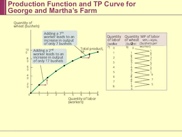
- 5. Production Function and TP Curve for George and Martha’s Farm 0 1 2 3 4 5
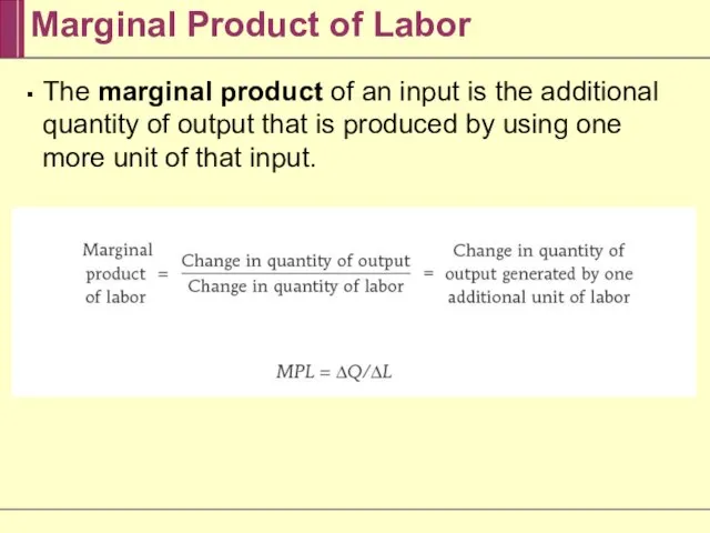
- 6. The marginal product of an input is the additional quantity of output that is produced by
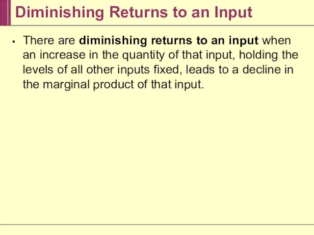
- 7. Diminishing Returns to an Input There are diminishing returns to an input when an increase in
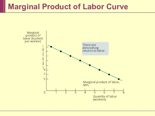
- 8. Marginal Product of Labor Curve Marginal product of labor, MPL 7 8 6 5 4 3
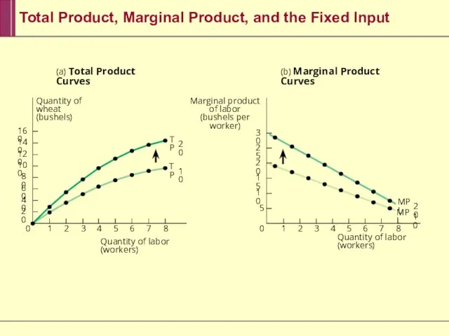
- 9. (a) Total Product Curves (b) Marginal Product Curves Marginal product of labor (bushels per worker) Quantity
- 10. From the Production Function to Cost Curves A fixed cost is a cost that does not
- 11. Total Cost Curve The total cost of producing a given quantity of output is the sum
- 12. Total Cost Curve for George and Martha’s Farm 19 36 51 64 75 84 91 96
- 13. The Mythical Man-Month Quantity of labor (programmers) TP MPL 0 0 Quantity of labor (programmers) Marginal
- 14. Two Key Concepts: Marginal Cost and Average Cost As in the case of marginal product, marginal
- 15. Costs at Selena’s Gourmet Salsas
- 16. Total Cost and Marginal Cost Curves for Selena’s Gourmet Salsas $250 200 150 100 50 Cost
- 17. Why is the Marginal Cost Curve Upward Sloping? Because there are diminishing returns to inputs in
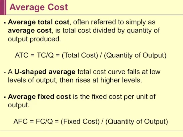
- 18. Average Cost Average total cost, often referred to simply as average cost, is total cost divided
- 19. Average Cost Average variable cost is the variable cost per unit of output. AVC = VC/Q=
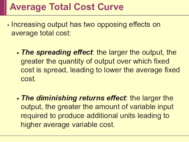
- 20. Average Total Cost Curve Increasing output has two opposing effects on average total cost: The spreading
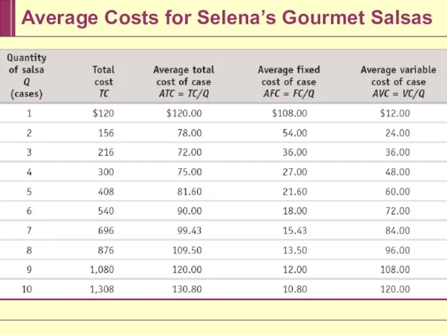
- 21. Average Costs for Selena’s Gourmet Salsas
- 22. Average Total Cost Curve for Selena’s Gourmet Salsas Average total cost, ATC M 7 8 9
- 23. Putting the Four Cost Curves Together Note that: Marginal cost is upward sloping due to diminishing
- 24. Marginal Cost and Average Cost Curves for Selena’s Gourmet Salsas $250 200 150 100 50 7
- 25. General Principles That Are Always True About a Firm’s Marginal and Average Total Cost Curves The
- 26. The Relationship Between the Average Total Cost and the Marginal Cost Curves Cost of unit Quantity
- 27. Does the Marginal Cost Curve Always Slope Upward? In practice, marginal cost curves often slope downward
- 28. More Realistic Cost Curves MC A T C A VC Cost of unit Quantity 2. …
- 29. Short-Run versus Long-Run Costs In the short run, fixed cost is completely outside the control of
- 30. Choosing the Level of Fixed Cost of Selena’s Gourmet Salsas $250 200 150 100 50 Cost
- 31. The long-run average total cost curve shows the relationship between output and average total cost when
- 32. Short-Run and Long-Run Average Total Cost Curves B A T C 6 A T C 9
- 33. Returns to Scale There are increasing returns to scale (economies of scale) when long-run average total
- 34. The relationship between inputs and output is a producer’s production function. In the short run, the
- 35. Average total cost, total cost divided by quantity of output, is the cost of the average
- 37. Скачать презентацию
Слайд 3The Production Function
A production function is the relationship between the quantity of
The Production Function
A production function is the relationship between the quantity of
Слайд 4Inputs and Output
The long run is the time period in which all
Inputs and Output
The long run is the time period in which all
Слайд 5Production Function and TP Curve for
George and Martha’s Farm
0
1
2
3
4
5
6
7
8
19
17
15
13
11
9
7
5
0
19
36
51
64
75
84
91
96
Quantity of labor L
(worker)
Quantity
Production Function and TP Curve for
George and Martha’s Farm
0
1
2
3
4
5
6
7
8
19
17
15
13
11
9
7
5
0
19
36
51
64
75
84
91
96
Quantity of labor L
(worker)
Quantity
Слайд 6The marginal product of an input is the additional quantity of output
The marginal product of an input is the additional quantity of output
Слайд 7Diminishing Returns to an Input
There are diminishing returns to an input when
Diminishing Returns to an Input
There are diminishing returns to an input when
Слайд 8Marginal Product of Labor Curve
Marginal product of labor, MPL
7
8
6
5
4
3
2
1
0
19
17
15
13
11
9
7
5
Marginal product of labor
Marginal Product of Labor Curve
Marginal product of labor, MPL
7
8
6
5
4
3
2
1
0
19
17
15
13
11
9
7
5
Marginal product of labor
Слайд 9(a) Total Product Curves
(b) Marginal Product Curves
Marginal product of labor
(bushels per
(a) Total Product Curves
(b) Marginal Product Curves
Marginal product of labor
(bushels per
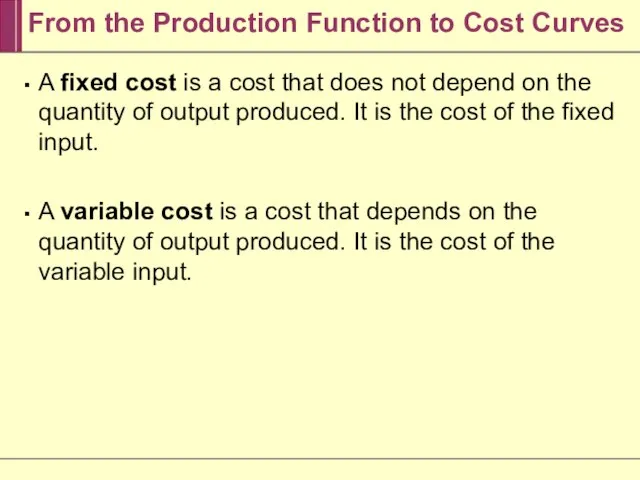
Слайд 10From the Production Function to Cost Curves
A fixed cost is a cost
From the Production Function to Cost Curves
A fixed cost is a cost
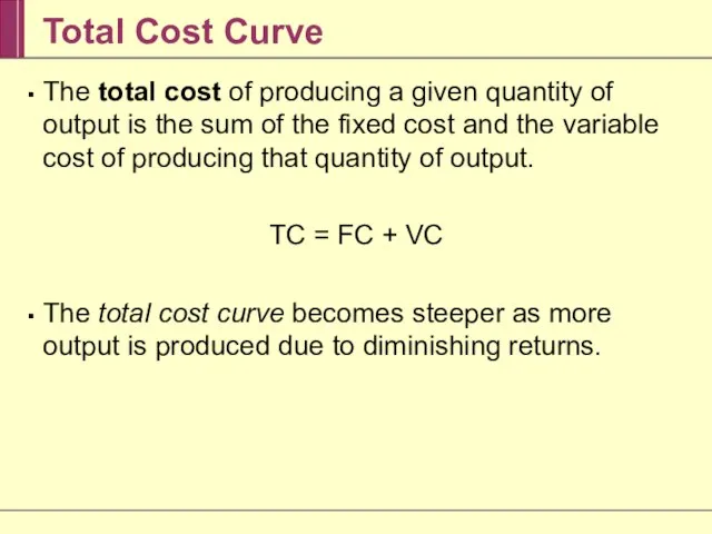
Слайд 11Total Cost Curve
The total cost of producing a given quantity of output
Total Cost Curve
The total cost of producing a given quantity of output
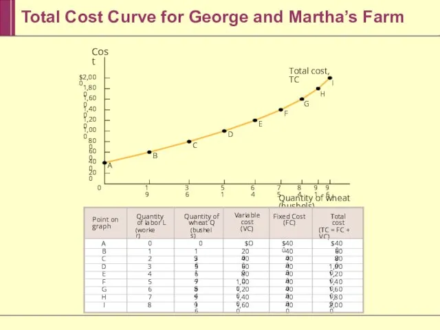
Слайд 12Total Cost Curve for George and Martha’s Farm
19
36
51
64
75
84
91
96
0
$2,000
1,800
1,600
1,400
1,200
1,000
800
600
400
200
Cost
Quantity of wheat (bushels)
A
B
C
D
E
F
G
Total cost,
Total Cost Curve for George and Martha’s Farm
19
36
51
64
75
84
91
96
0
$2,000
1,800
1,600
1,400
1,200
1,000
800
600
400
200
Cost
Quantity of wheat (bushels)
A
B
C
D
E
F
G
Total cost,
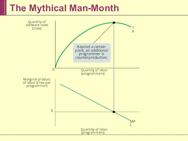
Слайд 13The Mythical Man-Month
Quantity of labor (programmers)
TP
MPL
0
0
Quantity of labor (programmers)
Marginal product of labor
The Mythical Man-Month
Quantity of labor (programmers)
TP
MPL
0
0
Quantity of labor (programmers)
Marginal product of labor
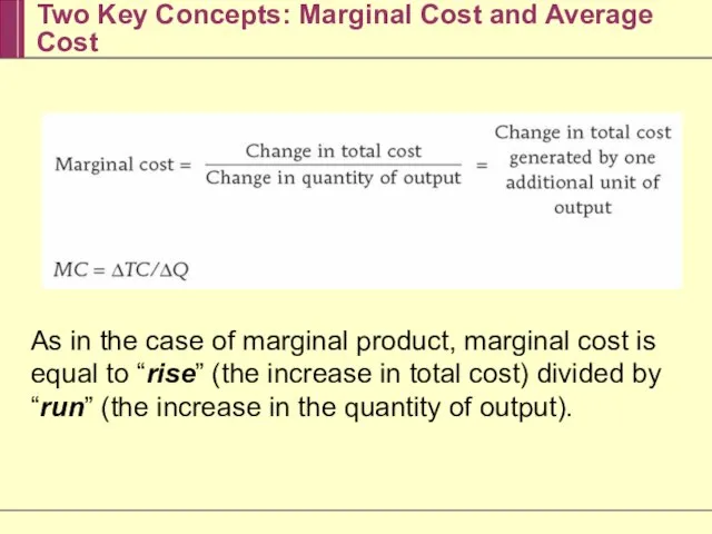
Слайд 14Two Key Concepts: Marginal Cost and Average Cost
As in the case of
Two Key Concepts: Marginal Cost and Average Cost
As in the case of
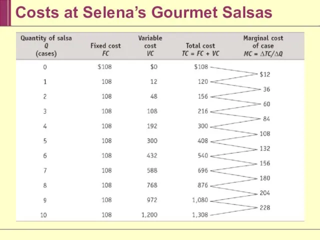
Слайд 15Costs at Selena’s Gourmet Salsas
Costs at Selena’s Gourmet Salsas
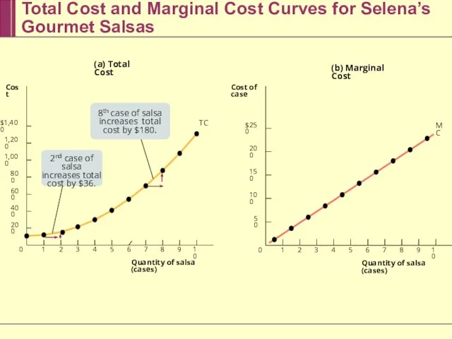
Слайд 16Total Cost and Marginal Cost Curves for Selena’s Gourmet Salsas
$250
200
150
100
50
Cost of case
7
8
9
10
6
5
4
3
2
1
0
$1,400
1,200
1,000
800
600
400
200
Cost
Quantity
Total Cost and Marginal Cost Curves for Selena’s Gourmet Salsas
$250
200
150
100
50
Cost of case
7
8
9
10
6
5
4
3
2
1
0
$1,400
1,200
1,000
800
600
400
200
Cost
Quantity
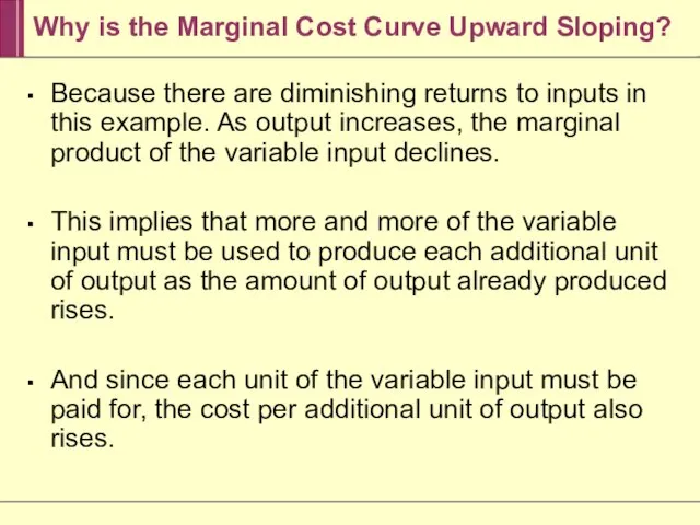
Слайд 17Why is the Marginal Cost Curve Upward Sloping?
Because there are diminishing returns
Why is the Marginal Cost Curve Upward Sloping?
Because there are diminishing returns
Слайд 18Average Cost
Average total cost, often referred to simply as average cost, is
Average Cost
Average total cost, often referred to simply as average cost, is
Слайд 19Average Cost
Average variable cost is the variable cost per unit of output.
Average Cost
Average variable cost is the variable cost per unit of output.
Слайд 20Average Total Cost Curve
Increasing output has two opposing effects on average total
Average Total Cost Curve
Increasing output has two opposing effects on average total
Слайд 21Average Costs for Selena’s Gourmet Salsas
Average Costs for Selena’s Gourmet Salsas
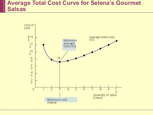
Слайд 22Average Total Cost Curve for Selena’s Gourmet Salsas
Average total cost, ATC
M
7
8
9
10
6
5
4
3
2
1
0
$140
120
100
80
60
40
20
Minimum average
Average Total Cost Curve for Selena’s Gourmet Salsas
Average total cost, ATC
M
7
8
9
10
6
5
4
3
2
1
0
$140
120
100
80
60
40
20
Minimum average
Слайд 23Putting the Four Cost Curves Together
Note that:
Marginal cost is upward sloping due
Putting the Four Cost Curves Together
Note that:
Marginal cost is upward sloping due
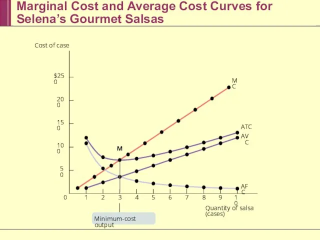
Слайд 24Marginal Cost and Average Cost Curves for Selena’s Gourmet Salsas
$250
200
150
100
50
7
8
9
10
6
5
4
3
2
1
M
0
MC
A
T
C
A
VC
AFC
Minimum-cost output
Cost of
Marginal Cost and Average Cost Curves for Selena’s Gourmet Salsas
$250
200
150
100
50
7
8
9
10
6
5
4
3
2
1
M
0
MC
A
T
C
A
VC
AFC
Minimum-cost output
Cost of
Слайд 25General Principles That Are Always True About a Firm’s Marginal and Average
General Principles That Are Always True About a Firm’s Marginal and Average
Слайд 26The Relationship Between the Average Total Cost and the Marginal Cost Curves
Cost
The Relationship Between the Average Total Cost and the Marginal Cost Curves
Cost
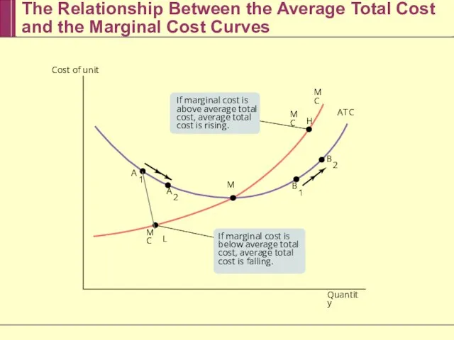
Слайд 27Does the Marginal Cost Curve Always Slope Upward?
In practice, marginal cost curves
Does the Marginal Cost Curve Always Slope Upward?
In practice, marginal cost curves
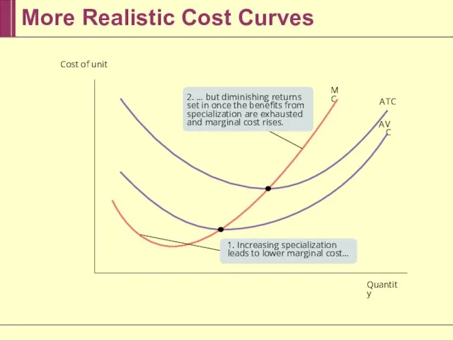
Слайд 28More Realistic Cost Curves
MC
A
T
C
A
VC
Cost of unit
Quantity
2. … but diminishing returns set in
More Realistic Cost Curves
MC
A
T
C
A
VC
Cost of unit
Quantity
2. … but diminishing returns set in
Слайд 29Short-Run versus Long-Run Costs
In the short run, fixed cost is completely outside
Short-Run versus Long-Run Costs
In the short run, fixed cost is completely outside
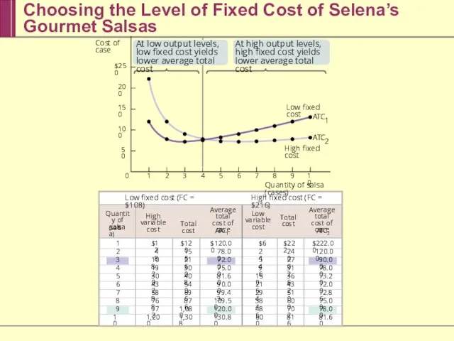
Слайд 30Choosing the Level of Fixed Cost of Selena’s Gourmet Salsas
$250
200
150
100
50
Cost of case
Quantity
Choosing the Level of Fixed Cost of Selena’s Gourmet Salsas
$250
200
150
100
50
Cost of case
Quantity
Слайд 31The long-run average total cost curve shows the relationship between output and
The long-run average total cost curve shows the relationship between output and
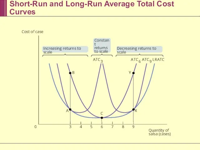
Слайд 32Short-Run and Long-Run Average Total Cost Curves
B
A
T
C
6
A
T
C
9
A
T
C
3
L
R
A
T
C
3
5
8
4
7
0
6
9
Increasing returns to scale
Decreasing returns to
Short-Run and Long-Run Average Total Cost Curves
B
A
T
C
6
A
T
C
9
A
T
C
3
L
R
A
T
C
3
5
8
4
7
0
6
9
Increasing returns to scale
Decreasing returns to
Слайд 33Returns to Scale
There are increasing returns to scale (economies of scale) when
Returns to Scale
There are increasing returns to scale (economies of scale) when
Слайд 34The relationship between inputs and output is a producer’s production function. In
The relationship between inputs and output is a producer’s production function. In
Слайд 35Average total cost, total cost divided by quantity of output, is the
Average total cost, total cost divided by quantity of output, is the
 Итоговая аттестация пилотного класса в рамках реализации ФГОС НОО
 Достоевский Ф.М
 Вредные привычки у детей. Консультация для родителей
 ТКС
ТКС Измерение удельной теплоемкости твердого тела
 «Деревня…
 Церкви Ленинграда в годы Советской власти
 Условия и механизмы функционирования рынка информационных услуг и продуктов
 Презентация на тему Жизнь и творчество И.К. Айвазовского
 Это – Кинематограф!
 Классификация видов групп однородной продукции и их характеристики
 Погрузочно-доставочная машина LH514L
 Удивительная
 Лекция 3 Общение как социально-психологический механизм
 Организация и техническое оснащение работ по приготовлению, хранению, подготовке к реализации горячих соусов
 Кривая Филлипса: выбор между безработицей и инфляцией
 ГИА по русскому языку
 Тема 5 (Форми дежави)
 собственность эк 11
 Найбільші біржі світу. 9 клас
 АЙСБЕРГ
 Система оценки эффективности исполнителя и удовлетворенности клиента качеством сервиса по выполненным заявкам
 Product Placement
 Мои жизненные ценности
 2022-10-6 Резолюция № 1 (1)
 Классические технологии хитрости на экзамене
 Презентация на тему Освоение культурного наследия Многоканальная модель освоения культурного наследия
  Malsharuashylyq