- Acoustic Waveform Processing

Содержание
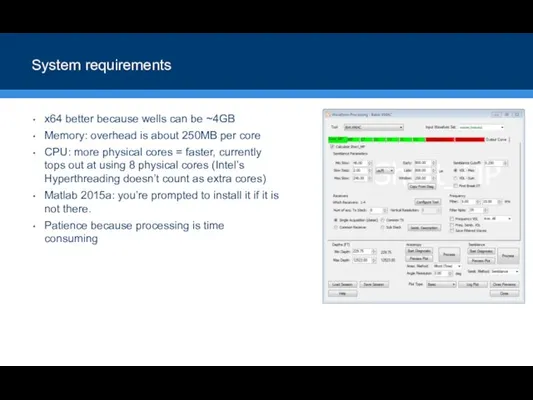
- 2. System requirements x64 better because wells can be ~4GB Memory: overhead is about 250MB per core
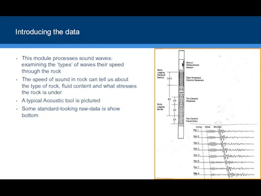
- 3. Introducing the data This module processes sound waves: examining the ‘types’ of waves their speed through
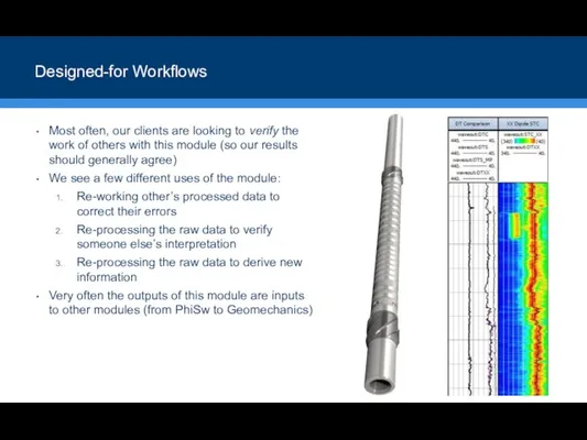
- 4. Designed-for Workflows Most often, our clients are looking to verify the work of others with this
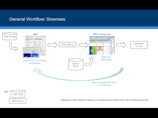
- 5. General Workflow: Slowness Slowness curves STC (VDLs) AWP Raw Waves Vendor STCs AWP: Picking tool From
- 6. General Workflow: Anisotropy Dispersion Outputs Anisotropy Map AWP Raw Waves From DLIS AWP output Key: User
- 7. WORKFLOW 1: RE-PICKING Slowness from other people’s processing Slowness curves STC (VDLs) AWP Raw Waves Vendor
- 8. Workflow 1: “Re-picking” Re-working other’s processed data to correct their errors The most trivial use of
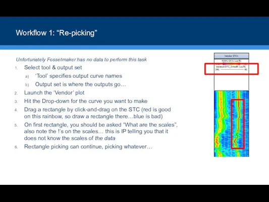
- 9. Workflow 1: “Re-picking” Unfortunately Fossetmaker has no data to perform this task Select tool & output
- 10. Workflow 1: “Re-picking” Unfortunately Fossetmaker has no data to perform this task Select tool & output
- 11. Workflow 1: “Re-picking” Unfortunately Fossetmaker has no data to perform this task Select tool & output
- 12. Workflow 1: “Re-picking” Unfortunately Fossetmaker has no data to perform this task Select tool & output
- 13. Workflow 1: “Re-picking” Unfortunately Fossetmaker has no data to perform this task Select tool & output
- 14. Workflow 1: “Re-picking” Unfortunately Fossetmaker has no data to perform this task Select tool & output
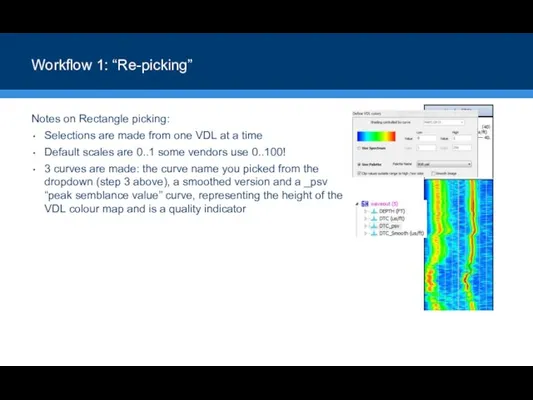
- 15. Workflow 1: “Re-picking” Notes on Rectangle picking: Selections are made from one VDL at a time
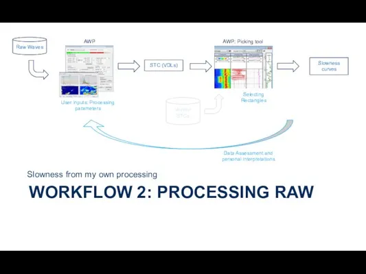
- 16. WORKFLOW 2: PROCESSING RAW Slowness from my own processing Slowness curves STC (VDLs) AWP Raw Waves
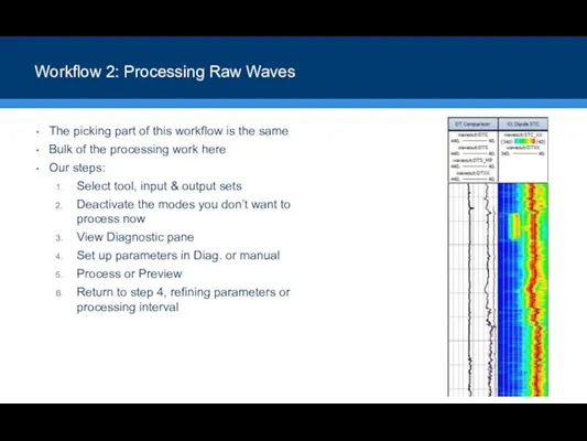
- 17. Workflow 2: Processing Raw Waves The picking part of this workflow is the same Bulk of
- 18. Workflow 2: Processing Raw Waves Select tool, input & output set ‘Tool’ specifies the ‘modes’ (Short_MP,
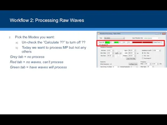
- 19. Workflow 2: Processing Raw Waves Pick the Modes you want: Un-check the “Calculate ??” to turn
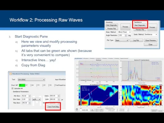
- 20. Workflow 2: Processing Raw Waves Start Diagnostic Pane Here we view and modify processing parameters visually
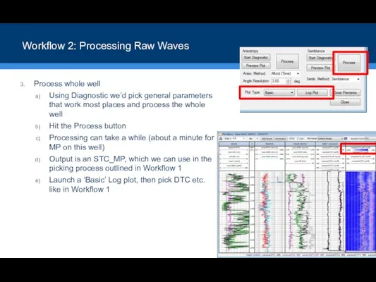
- 21. Workflow 2: Processing Raw Waves Process whole well Using Diagnostic we’d pick general parameters that work
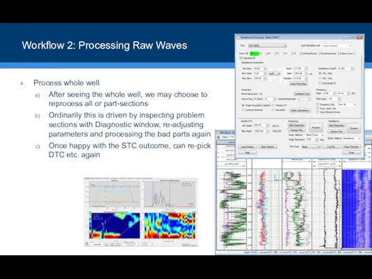
- 22. Workflow 2: Processing Raw Waves Process whole well After seeing the whole well, we may choose
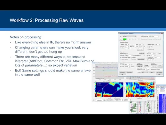
- 23. Workflow 2: Processing Raw Waves Notes on processing: Like everything else in IP, there’s no ‘right’
- 24. WORKFLOW 3: ANISOTROPY Azimuthally changing slowess Dispersion Outputs Anisotropy Map AWP Raw Waves User inputs: Anisotropy
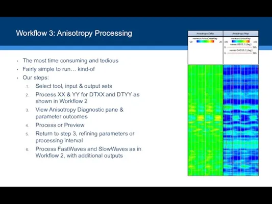
- 25. Workflow 3: Anisotropy Processing The most time consuming and tedious Fairly simple to run… kind-of Our
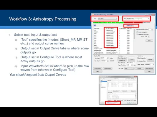
- 26. Workflow 3: Anisotropy Processing Select tool, input & output set ‘Tool’ specifies the ‘modes’ (Short_MP, MP,
- 27. Workflow 3: Anisotropy Processing Process XX & YY for DTXX and DTYY Using Workflow 2 you
- 28. Workflow 3: Anisotropy Processing Inspect the Diagnostic Window for Anisotropy This shows all the waveforms used,
- 29. Workflow 3: Anisotropy Processing Process for Anisotropy This takes a long time! A very long time!
- 30. Workflow 3: Anisotropy Processing Refine parameters Parameters used for Anisotropy come from the XX tab Use
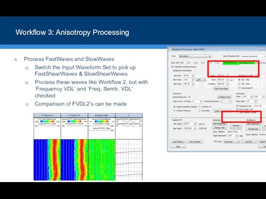
- 31. Workflow 3: Anisotropy Processing Process FastWaves and SlowWaves Switch the Input Waveform Set to pick up
- 33. Скачать презентацию
Слайд 3Introducing the data
This module processes sound waves: examining the ‘types’ of waves
Introducing the data
This module processes sound waves: examining the ‘types’ of waves
Слайд 4Designed-for Workflows
Most often, our clients are looking to verify the work of
Designed-for Workflows
Most often, our clients are looking to verify the work of
Слайд 5General Workflow: Slowness
Slowness curves
STC (VDLs)
AWP
Raw Waves
Vendor STCs
AWP: Picking tool
From DLIS
AWP output
Key:
User inputs:
General Workflow: Slowness
Slowness curves
STC (VDLs)
AWP
Raw Waves
Vendor STCs
AWP: Picking tool
From DLIS
AWP output
Key:
User inputs:
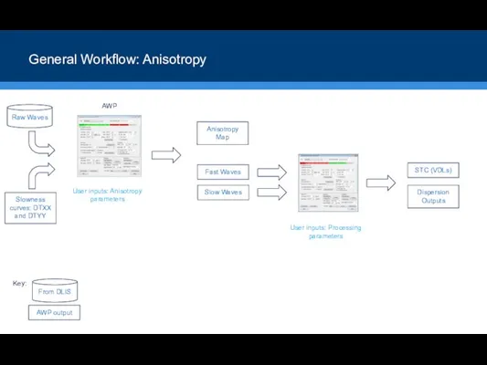
Слайд 6General Workflow: Anisotropy
Dispersion Outputs
Anisotropy Map
AWP
Raw Waves
From DLIS
AWP output
Key:
User inputs: Anisotropy parameters
Slowness curves:
General Workflow: Anisotropy
Dispersion Outputs
Anisotropy Map
AWP
Raw Waves
From DLIS
AWP output
Key:
User inputs: Anisotropy parameters
Slowness curves:
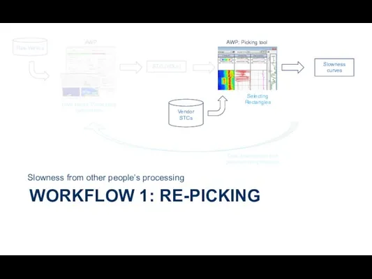
Слайд 7WORKFLOW 1: RE-PICKING
Slowness from other people’s processing
Slowness curves
STC (VDLs)
AWP
Raw Waves
Vendor STCs
AWP: Picking
WORKFLOW 1: RE-PICKING
Slowness from other people’s processing
Slowness curves
STC (VDLs)
AWP
Raw Waves
Vendor STCs
AWP: Picking
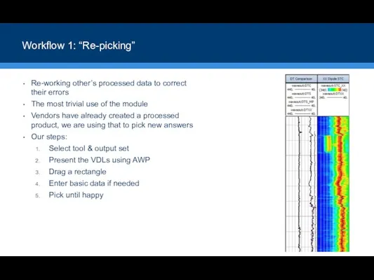
Слайд 8Workflow 1: “Re-picking”
Re-working other’s processed data to correct their errors
The most trivial
Workflow 1: “Re-picking”
Re-working other’s processed data to correct their errors
The most trivial
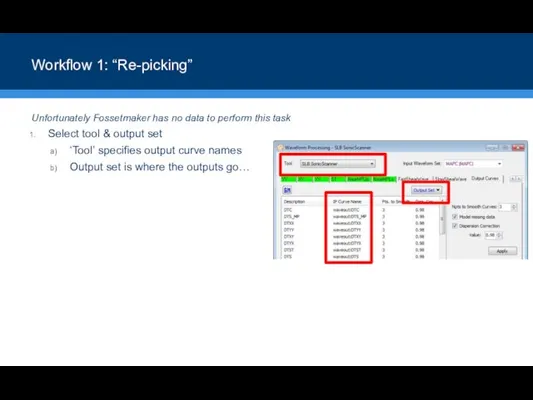
Слайд 9Workflow 1: “Re-picking”
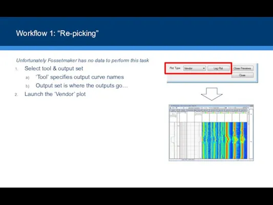
Unfortunately Fossetmaker has no data to perform this task
Select tool
Workflow 1: “Re-picking”
Unfortunately Fossetmaker has no data to perform this task
Select tool
Слайд 10Workflow 1: “Re-picking”
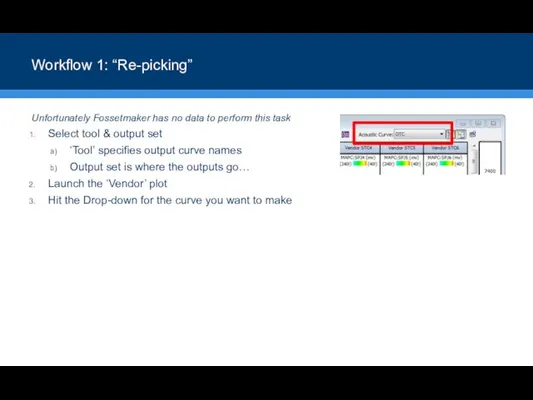
Unfortunately Fossetmaker has no data to perform this task
Select tool
Workflow 1: “Re-picking”
Unfortunately Fossetmaker has no data to perform this task
Select tool
Слайд 11Workflow 1: “Re-picking”
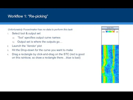
Unfortunately Fossetmaker has no data to perform this task
Select tool
Workflow 1: “Re-picking”
Unfortunately Fossetmaker has no data to perform this task
Select tool
Слайд 12Workflow 1: “Re-picking”
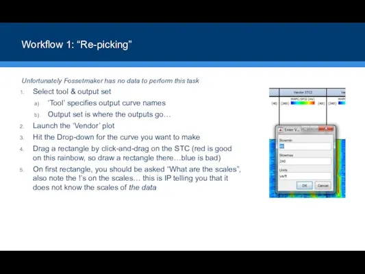
Unfortunately Fossetmaker has no data to perform this task
Select tool
Workflow 1: “Re-picking”
Unfortunately Fossetmaker has no data to perform this task
Select tool
Слайд 13Workflow 1: “Re-picking”
Unfortunately Fossetmaker has no data to perform this task
Select tool
Workflow 1: “Re-picking”
Unfortunately Fossetmaker has no data to perform this task
Select tool
Слайд 14Workflow 1: “Re-picking”
Unfortunately Fossetmaker has no data to perform this task
Select tool
Workflow 1: “Re-picking”
Unfortunately Fossetmaker has no data to perform this task
Select tool
Слайд 15Workflow 1: “Re-picking”
Notes on Rectangle picking:
Selections are made from one VDL at
Workflow 1: “Re-picking”
Notes on Rectangle picking:
Selections are made from one VDL at
Слайд 16WORKFLOW 2: PROCESSING RAW
Slowness from my own processing
Slowness curves
STC (VDLs)
AWP
Raw Waves
Vendor STCs
AWP:
WORKFLOW 2: PROCESSING RAW
Slowness from my own processing
Slowness curves
STC (VDLs)
AWP
Raw Waves
Vendor STCs
AWP:
Слайд 17Workflow 2: Processing Raw Waves
The picking part of this workflow is the
Workflow 2: Processing Raw Waves
The picking part of this workflow is the
Слайд 18Workflow 2: Processing Raw Waves
Select tool, input & output set
‘Tool’ specifies the
Workflow 2: Processing Raw Waves
Select tool, input & output set
‘Tool’ specifies the

Слайд 19Workflow 2: Processing Raw Waves
Pick the Modes you want:
Un-check the “Calculate ??”
Workflow 2: Processing Raw Waves
Pick the Modes you want:
Un-check the “Calculate ??”
Слайд 20Workflow 2: Processing Raw Waves
Start Diagnostic Pane
Here we view and modify processing
Workflow 2: Processing Raw Waves
Start Diagnostic Pane
Here we view and modify processing
Слайд 21Workflow 2: Processing Raw Waves
Process whole well
Using Diagnostic we’d pick general parameters
Workflow 2: Processing Raw Waves
Process whole well
Using Diagnostic we’d pick general parameters
Слайд 22Workflow 2: Processing Raw Waves
Process whole well
After seeing the whole well, we
Workflow 2: Processing Raw Waves
Process whole well
After seeing the whole well, we
Слайд 23Workflow 2: Processing Raw Waves
Notes on processing:
Like everything else in IP, there’s
Workflow 2: Processing Raw Waves
Notes on processing:
Like everything else in IP, there’s
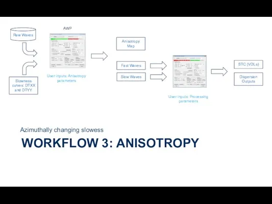
Слайд 24WORKFLOW 3: ANISOTROPY
Azimuthally changing slowess
Dispersion Outputs
Anisotropy Map
AWP
Raw Waves
User inputs: Anisotropy parameters
Slowness curves:
WORKFLOW 3: ANISOTROPY
Azimuthally changing slowess
Dispersion Outputs
Anisotropy Map
AWP
Raw Waves
User inputs: Anisotropy parameters
Slowness curves:
Слайд 25Workflow 3: Anisotropy Processing
The most time consuming and tedious
Fairly simple to run…
Workflow 3: Anisotropy Processing
The most time consuming and tedious
Fairly simple to run…
Слайд 26Workflow 3: Anisotropy Processing
Select tool, input & output set
‘Tool’ specifies the ‘modes’
Workflow 3: Anisotropy Processing
Select tool, input & output set
‘Tool’ specifies the ‘modes’
Слайд 27Workflow 3: Anisotropy Processing
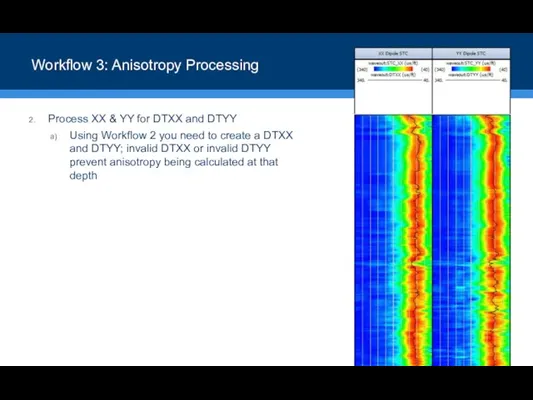
Process XX & YY for DTXX and DTYY
Using Workflow
Workflow 3: Anisotropy Processing
Process XX & YY for DTXX and DTYY
Using Workflow
Слайд 28Workflow 3: Anisotropy Processing
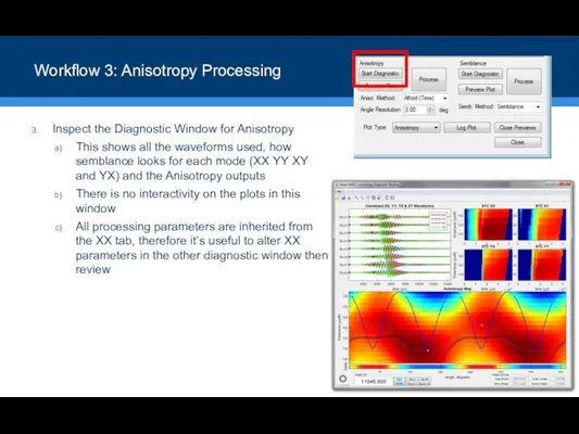
Inspect the Diagnostic Window for Anisotropy
This shows all the
Workflow 3: Anisotropy Processing
Inspect the Diagnostic Window for Anisotropy
This shows all the
Слайд 29Workflow 3: Anisotropy Processing
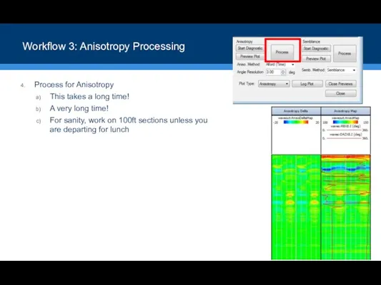
Process for Anisotropy
This takes a long time!
A very long
Workflow 3: Anisotropy Processing
Process for Anisotropy
This takes a long time!
A very long
Слайд 30Workflow 3: Anisotropy Processing
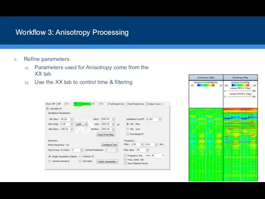
Refine parameters
Parameters used for Anisotropy come from the XX
Workflow 3: Anisotropy Processing
Refine parameters
Parameters used for Anisotropy come from the XX
Слайд 31Workflow 3: Anisotropy Processing
Process FastWaves and SlowWaves
Switch the Input Waveform Set to
Workflow 3: Anisotropy Processing
Process FastWaves and SlowWaves
Switch the Input Waveform Set to
 What’s the capital city?
 Animal - Zoo
 Molle's House
 September 11 attacks
 Презентация на тему The Boston Tea Party
  Verb to be
 Health Unit 8
 Food
Food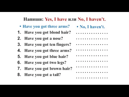 Напиши: Yes, I have или No, I haven't. (задание)
 Colors word search
 Smack
Smack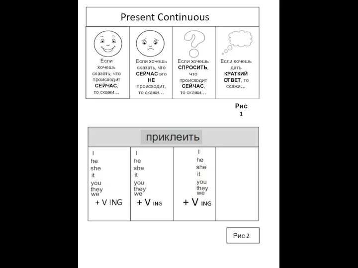 Present continuous
 Types of business letters
 Понимание английского языка через образное восприятие
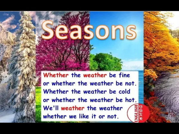 What season is it?
 We explain the way. Dialogue speech
 Презентация на тему Prince Andrew
  ABC holday
 This is a little Indian Girl
 Self Introduction
 Can-cant
 Short u
 Презентация на тему Welcome the United Kingdom of Great Britain and Northern Ireland
  A historical tour round old streets of Mikhaylovka
 Games. The vowels (a, e, i, o, u) have been removed from these words. Try to guess what each word is. Buildings & Places
 Reading toys
 In the, on the
 The University of Nottingham, England