- Excel

Содержание
- 2. PLAN TO GRIND UP • Mean• Standard error• Median• Mode• Standard deviation• Sample Variance• Kurtosis• Skewness•
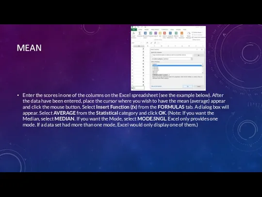
- 3. MEAN Enter the scores in one of the columns on the Excel spreadsheet (see the example
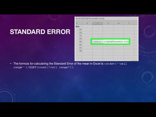
- 4. STANDARD ERROR The formula for calculating the Standard Error of the mean in Excel is =stdev(''cell
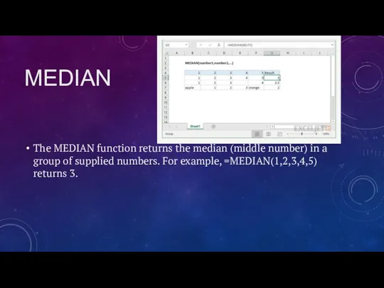
- 5. MEDIAN The MEDIAN function returns the median (middle number) in a group of supplied numbers. For
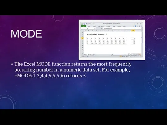
- 6. MODE The Excel MODE function returns the most frequently occurring number in a numeric data set.
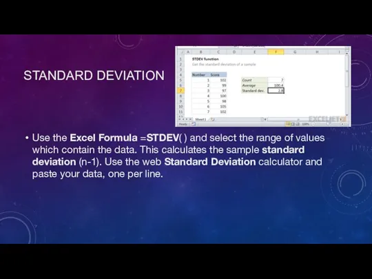
- 7. STANDARD DEVIATION Use the Excel Formula =STDEV( ) and select the range of values which contain
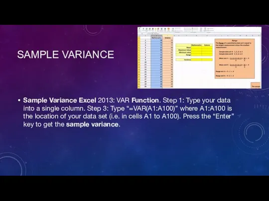
- 8. SAMPLE VARIANCE Sample Variance Excel 2013: VAR Function. Step 1: Type your data into a single
- 9. KURTOSIS KURT(number1, [number2], ...)The KURT function syntax has the following arguments:Number1, number2, ... Number1 is required,
- 10. SKEWNESS SKEW(number1, [number2], ...)The SKEW function syntax has the following arguments:Number1, number2, ... Number1 is required,
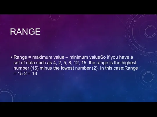
- 11. RANGE Range = maximum value – minimum valueSo if you have a set of data such
- 12. MAXIMUM =MAX (number1, [number2], ...)
- 13. MINIMUM =MIN (number1, [number2], ...)
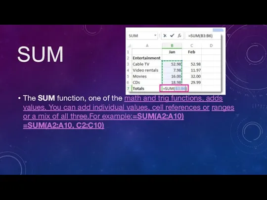
- 14. SUM The SUM function, one of the math and trig functions, adds values. You can add
- 16. Скачать презентацию

Слайд 3MEAN
Enter the scores in one of the columns on the Excel spreadsheet
MEAN
Enter the scores in one of the columns on the Excel spreadsheet
Слайд 4STANDARD ERROR
The formula for calculating the Standard Error of the mean in
STANDARD ERROR
The formula for calculating the Standard Error of the mean in
Слайд 5MEDIAN
The MEDIAN function returns the median (middle number) in a group of
MEDIAN
The MEDIAN function returns the median (middle number) in a group of
Слайд 6MODE
The Excel MODE function returns the most frequently occurring number in a numeric
MODE
The Excel MODE function returns the most frequently occurring number in a numeric
Слайд 7STANDARD DEVIATION
Use the Excel Formula =STDEV( ) and select the range of
STANDARD DEVIATION
Use the Excel Formula =STDEV( ) and select the range of
Слайд 8SAMPLE VARIANCE
Sample Variance Excel 2013: VAR Function. Step 1: Type your data
SAMPLE VARIANCE
Sample Variance Excel 2013: VAR Function. Step 1: Type your data
Слайд 9KURTOSIS
KURT(number1, [number2], ...)The KURT function syntax has the following arguments:Number1, number2, ... Number1
KURTOSIS
KURT(number1, [number2], ...)The KURT function syntax has the following arguments:Number1, number2, ... Number1
![KURTOSIS KURT(number1, [number2], ...)The KURT function syntax has the following arguments:Number1, number2,](/_ipx/f_webp&q_80&fit_contain&s_1440x1080/imagesDir/jpg/966825/slide-8.jpg)
Слайд 10SKEWNESS
SKEW(number1, [number2], ...)The SKEW function syntax has the following arguments:Number1, number2, ... Number1
SKEWNESS
SKEW(number1, [number2], ...)The SKEW function syntax has the following arguments:Number1, number2, ... Number1
![SKEWNESS SKEW(number1, [number2], ...)The SKEW function syntax has the following arguments:Number1, number2,](/_ipx/f_webp&q_80&fit_contain&s_1440x1080/imagesDir/jpg/966825/slide-9.jpg)
Слайд 11RANGE
Range = maximum value – minimum valueSo if you have a set
RANGE
Range = maximum value – minimum valueSo if you have a set
Слайд 12MAXIMUM
=MAX (number1, [number2], ...)
MAXIMUM
=MAX (number1, [number2], ...)
![MAXIMUM =MAX (number1, [number2], ...)](/_ipx/f_webp&q_80&fit_contain&s_1440x1080/imagesDir/jpg/966825/slide-11.jpg)
Слайд 13MINIMUM
=MIN (number1, [number2], ...)
MINIMUM
=MIN (number1, [number2], ...)
![MINIMUM =MIN (number1, [number2], ...)](/_ipx/f_webp&q_80&fit_contain&s_1440x1080/imagesDir/jpg/966825/slide-12.jpg)
Слайд 14SUM
The SUM function, one of the math and trig functions, adds values.
SUM
The SUM function, one of the math and trig functions, adds values.
 Present perfect. Simple activities
 What are they doing
 Christmas Jokes
 F.A.I.L. Means First Attempt In Learning
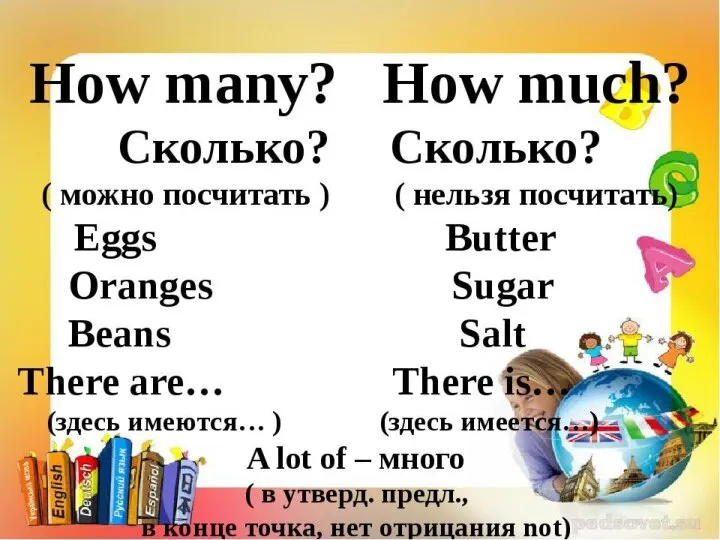 much many.Uncountable-неисчисляемый, Countable-исчисляемый
 Family and Friends. Holidays. Past Simple
 ДЗ для 10 кл. 10.10.22
 Have got (has got)
 Презентация на тему Здоровая и нездоровая пища
  My theme of dissertation is
 Animals fun activities games
 Questions template
 Указательные местоимения this – these / that - those
 Super Mario bros
 Dolch Vocabulary Words
 Times
Times Презентация на тему Favorite clothes (Любимая одежда)
  Slang
Slang Family. Who’s this?
 The new project
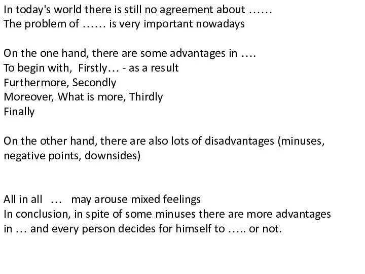 In today's world there is still
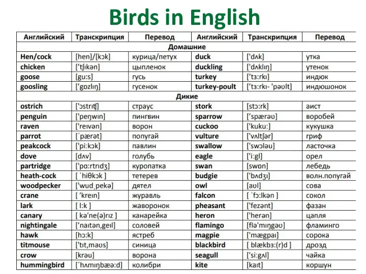 Birds in English
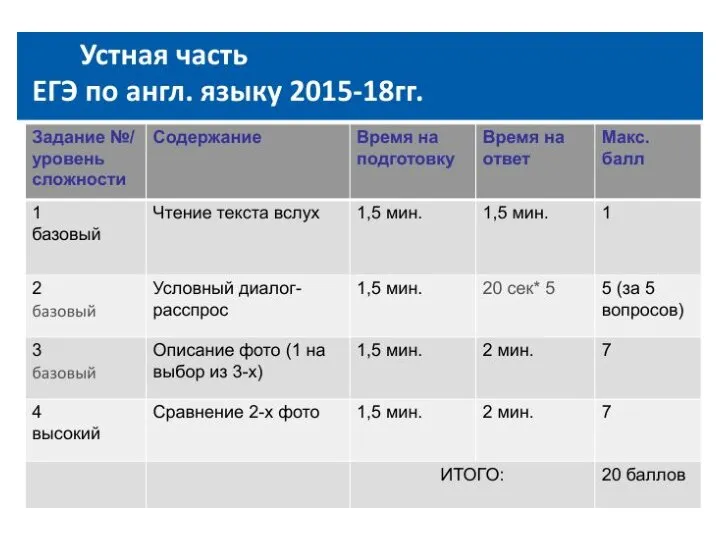 Устная часть ЭГЕ по английскому языку
 Внеклассное мероприятие. Holidays. Grammar
 Past Simple
 Presentation on Interesting facts about the Englishspeaking countries
 If + simple present
 Printed mass media