- Econometrics

Содержание
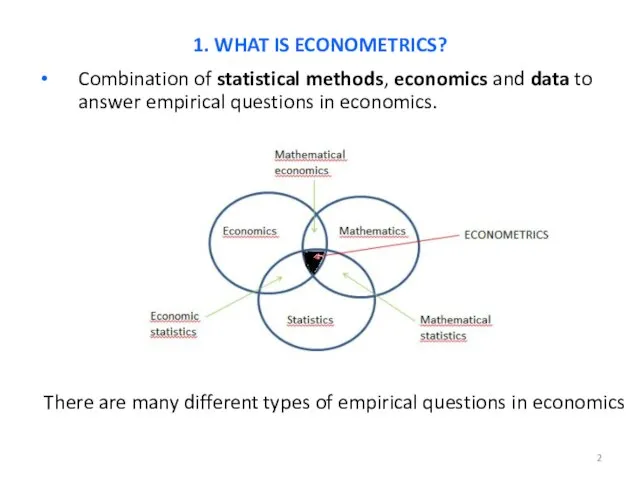
- 2. Combination of statistical methods, economics and data to answer empirical questions in economics. 1. WHAT IS
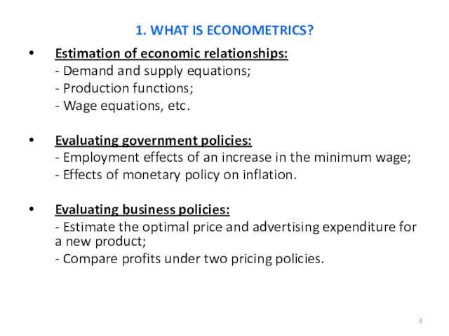
- 3. Estimation of economic relationships: - Demand and supply equations; - Production functions; - Wage equations, etc.
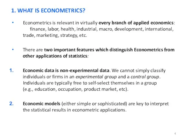
- 4. Econometrics is relevant in virtually every branch of applied economics: finance, labor, health, industrial, macro, development,
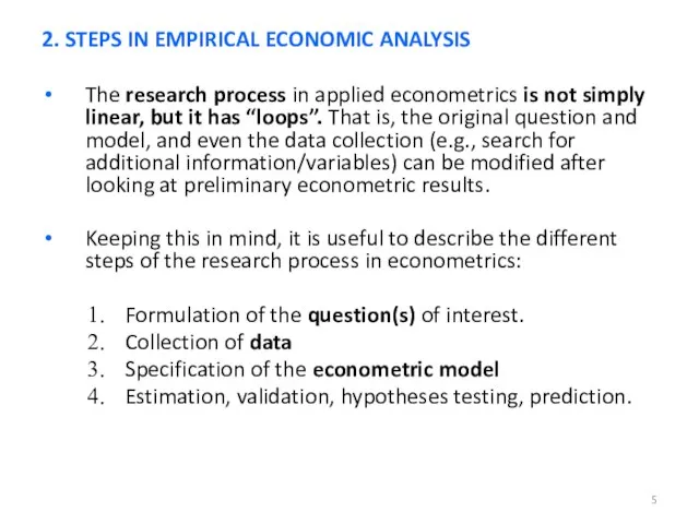
- 5. The research process in applied econometrics is not simply linear, but it has “loops”. That is,
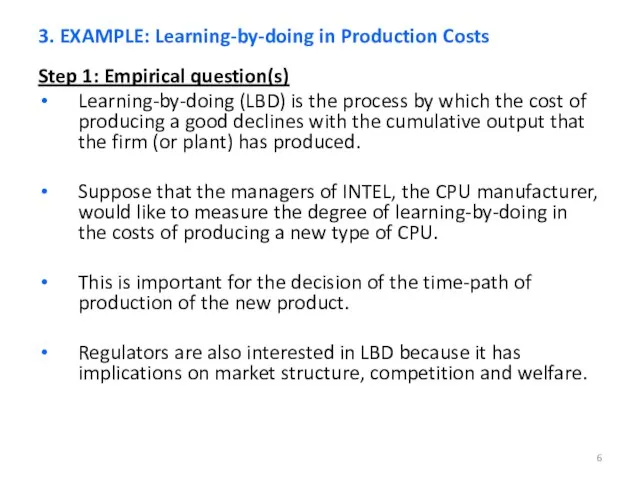
- 6. Step 1: Empirical question(s) Learning-by-doing (LBD) is the process by which the cost of producing a
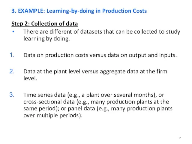
- 7. Step 2: Collection of data There are different of datasets that can be collected to study
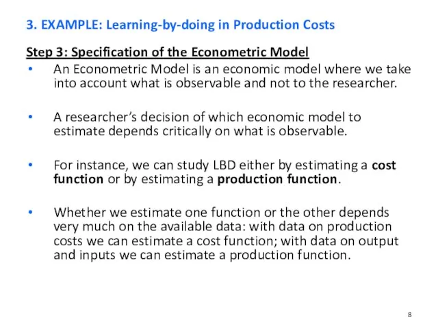
- 8. Step 3: Specification of the Econometric Model An Econometric Model is an economic model where we
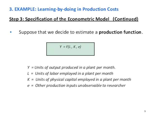
- 9. Step 3: Specification of the Econometric Model (Continued) Suppose that we decide to estimate a production
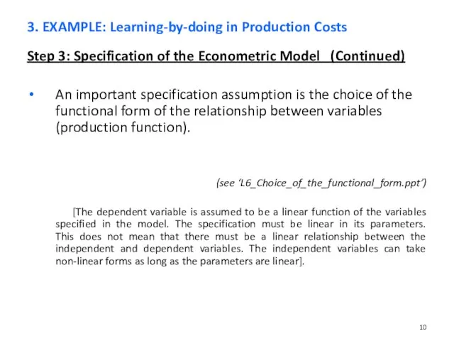
- 10. Step 3: Specification of the Econometric Model (Continued) An important specification assumption is the choice of
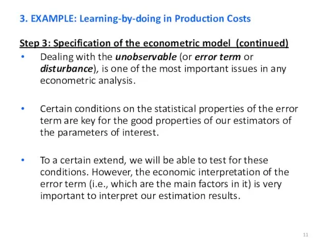
- 11. Step 3: Specification of the econometric model (continued) Dealing with the unobservable (or error term or
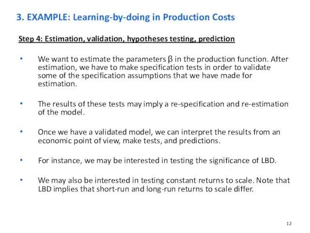
- 12. Step 4: Estimation, validation, hypotheses testing, prediction We want to estimate the parameters β in the
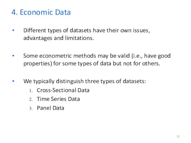
- 13. Different types of datasets have their own issues, advantages and limitations. Some econometric methods may be
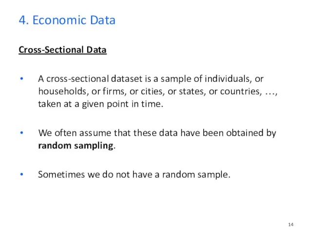
- 14. Cross-Sectional Data A cross-sectional dataset is a sample of individuals, or households, or firms, or cities,
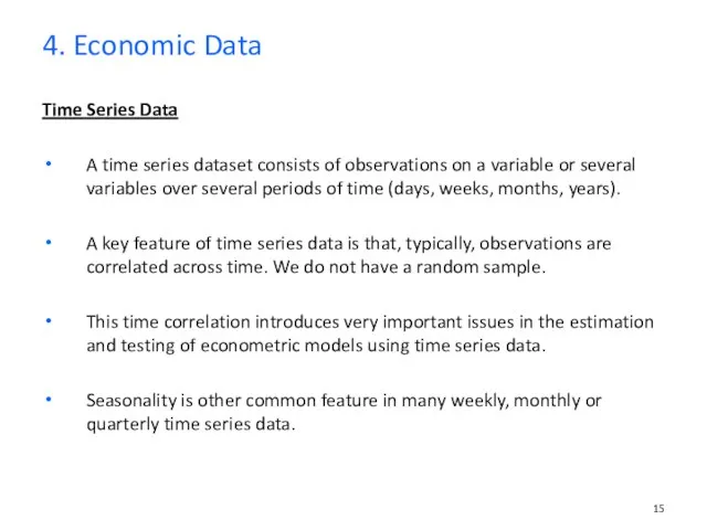
- 15. Time Series Data A time series dataset consists of observations on a variable or several variables
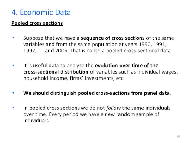
- 16. Pooled cross sections Suppose that we have a sequence of cross sections of the same variables
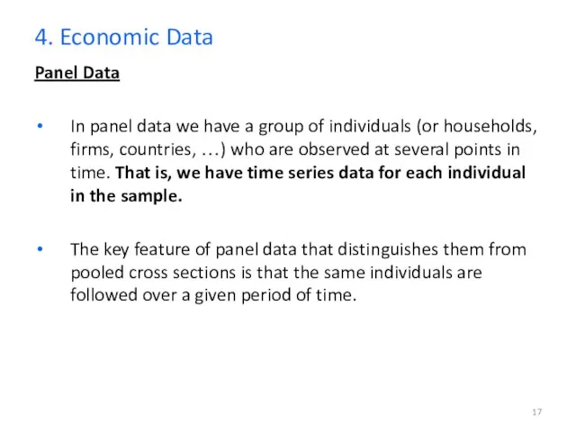
- 17. Panel Data In panel data we have a group of individuals (or households, firms, countries, …)
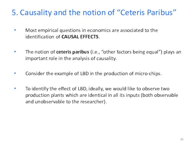
- 18. Most empirical questions in economics are associated to the identification of CAUSAL EFFECTS. The notion of
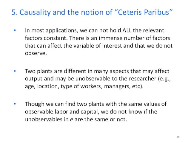
- 19. In most applications, we can not hold ALL the relevant factors constant. There is an immense
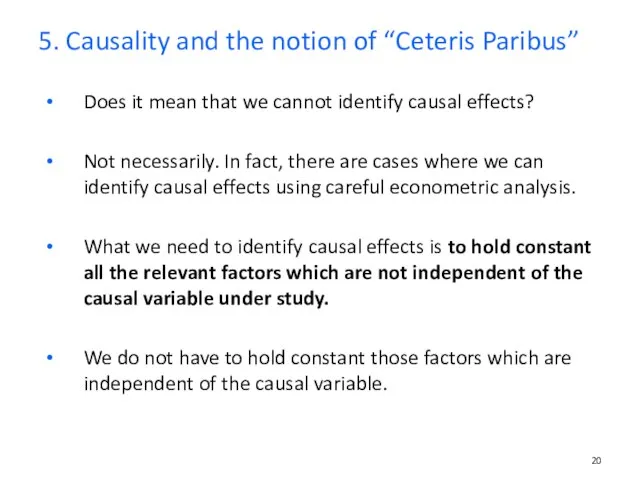
- 20. Does it mean that we cannot identify causal effects? Not necessarily. In fact, there are cases
- 21. We make two assumptions about the explanatory variables: The explanatory variables are not random variables We
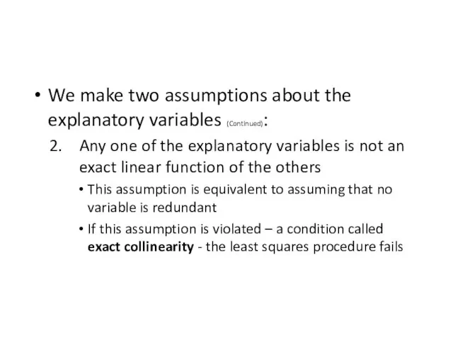
- 22. We make two assumptions about the explanatory variables (Continued): Any one of the explanatory variables is
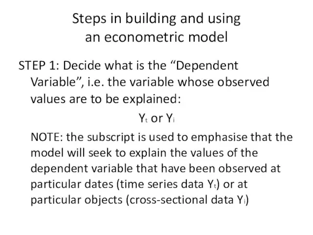
- 24. Steps in building and using an econometric model STEP 1: Decide what is the “Dependent Variable”,
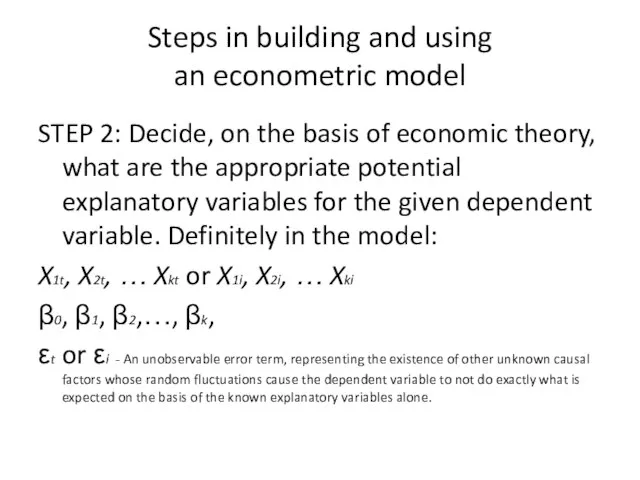
- 25. Steps in building and using an econometric model STEP 2: Decide, on the basis of economic
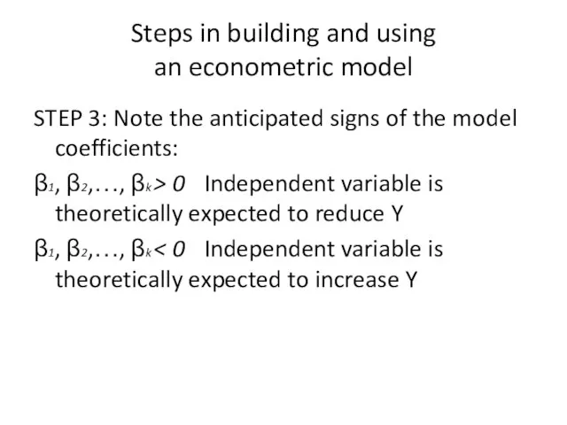
- 26. Steps in building and using an econometric model STEP 3: Note the anticipated signs of the
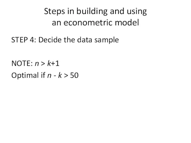
- 27. Steps in building and using an econometric model STEP 4: Decide the data sample NOTE: n
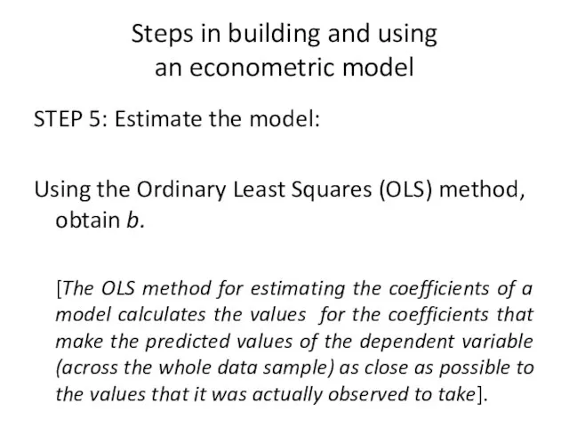
- 28. Steps in building and using an econometric model STEP 5: Estimate the model: Using the Ordinary
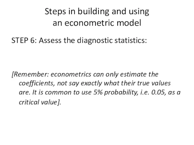
- 29. Steps in building and using an econometric model STEP 6: Assess the diagnostic statistics: [Remember: econometrics
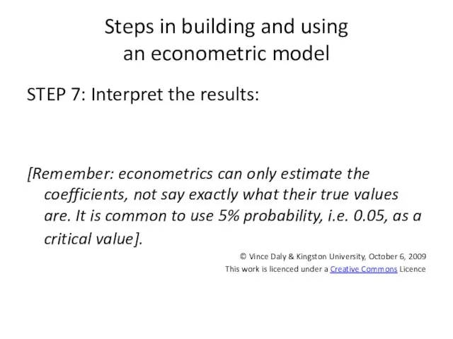
- 30. Steps in building and using an econometric model STEP 7: Interpret the results: [Remember: econometrics can
- 32. Скачать презентацию
Слайд 3Estimation of economic relationships:
- Demand and supply equations;
- Production functions;
- Wage
Estimation of economic relationships:
- Demand and supply equations;
- Production functions;
- Wage
Слайд 4Econometrics is relevant in virtually every branch of applied economics: finance, labor,
Econometrics is relevant in virtually every branch of applied economics: finance, labor,
Слайд 5The research process in applied econometrics is not simply linear, but it
The research process in applied econometrics is not simply linear, but it
Слайд 6Step 1: Empirical question(s)
Learning-by-doing (LBD) is the process by which the cost
Step 1: Empirical question(s)
Learning-by-doing (LBD) is the process by which the cost
Слайд 7Step 2: Collection of data
There are different of datasets that can be
Step 2: Collection of data
There are different of datasets that can be
Слайд 8Step 3: Specification of the Econometric Model
An Econometric Model is an economic
Step 3: Specification of the Econometric Model
An Econometric Model is an economic
Слайд 9Step 3: Specification of the Econometric Model (Continued)
Suppose that we decide
Step 3: Specification of the Econometric Model (Continued)
Suppose that we decide
Слайд 10Step 3: Specification of the Econometric Model (Continued)
An important specification assumption
Step 3: Specification of the Econometric Model (Continued)
An important specification assumption
Слайд 11Step 3: Specification of the econometric model (continued)
Dealing with the unobservable (or
Step 3: Specification of the econometric model (continued)
Dealing with the unobservable (or
Слайд 12Step 4: Estimation, validation, hypotheses testing, prediction
We want to estimate the parameters
Step 4: Estimation, validation, hypotheses testing, prediction
We want to estimate the parameters
Слайд 13Different types of datasets have their own issues, advantages and limitations.
Some econometric
Different types of datasets have their own issues, advantages and limitations.
Some econometric
Слайд 14Cross-Sectional Data
A cross-sectional dataset is a sample of individuals, or households, or
Cross-Sectional Data
A cross-sectional dataset is a sample of individuals, or households, or
Слайд 15Time Series Data
A time series dataset consists of observations on a variable
Time Series Data
A time series dataset consists of observations on a variable
Слайд 16Pooled cross sections
Suppose that we have a sequence of cross sections of
Pooled cross sections
Suppose that we have a sequence of cross sections of
Слайд 17Panel Data
In panel data we have a group of individuals (or households,
Panel Data
In panel data we have a group of individuals (or households,
Слайд 18Most empirical questions in economics are associated to the identification of CAUSAL
Most empirical questions in economics are associated to the identification of CAUSAL
Слайд 19In most applications, we can not hold ALL the relevant factors constant.
In most applications, we can not hold ALL the relevant factors constant.
Слайд 20Does it mean that we cannot identify causal effects?
Not necessarily. In
Does it mean that we cannot identify causal effects?
Not necessarily. In
Слайд 21We make two assumptions about the explanatory variables:
The explanatory variables are not
The explanatory variables are not
Слайд 22We make two assumptions about the explanatory variables (Continued):
Any one of
Any one of
Слайд 24
Steps in building and using
an econometric model
STEP 1: Decide what is
Steps in building and using
an econometric model
STEP 1: Decide what is
Слайд 25
Steps in building and using
an econometric model
STEP 2: Decide, on the
Steps in building and using
an econometric model
STEP 2: Decide, on the
Слайд 26
Steps in building and using
an econometric model
STEP 3: Note the anticipated
Steps in building and using
an econometric model
STEP 3: Note the anticipated
Слайд 27
Steps in building and using
an econometric model
STEP 4: Decide the data
Steps in building and using
an econometric model
STEP 4: Decide the data
Слайд 28
Steps in building and using
an econometric model
STEP 5: Estimate the model:
Using
Steps in building and using
an econometric model
STEP 5: Estimate the model:
Using
Слайд 29
Steps in building and using
an econometric model
STEP 6: Assess the diagnostic
Steps in building and using
an econometric model
STEP 6: Assess the diagnostic
Слайд 30
Steps in building and using
an econometric model
STEP 7: Interpret the results:
[Remember:
Steps in building and using
an econometric model
STEP 7: Interpret the results:
[Remember:
 ЭКОНОМИКА ПРИРОДОПОЛЬЗОВАНИЯ
 Заполнение формы 0503737. Отчет об исполнении учреждением плана его финансово-хозяйственной деятельности
 Капитализм в XVIII в. Промышленный переворот
 Наша мануфактура – это команда профессионалов. Нас объединяет жизненный оптимизм и желание изменить жизнь к лучшему. Мы ценим про
 ГБУ Озеленение и МОСЗЕЛЕНХОЗ
 Кружок "Ловкие пальчики"
 20220906___1__v3
 Инженерные войска Вооружённых Сил Российской Федерации
 Маркетинг в социальных сетях
 Динамика инцидентов
 3.6. Определение, прогнозирование и оценка риска
 Толерантность
  В наших выступлениях соединены самые искусные и эффектные виды фристайла: Футбольный фристайл (Чемпион России по версии Red Bull Street St
 Основные достижения Павла I
 Предмет, методология и задачи курса
 Механическое полирование
 Законодательное регулирование льготного социального обеспечения
 Одежда и обувь
 Центр Милтон по изучению юдаики
 Культура Тибета
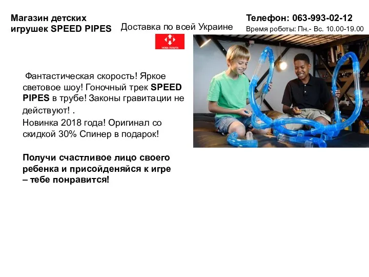 Магазин детских игрушек SPEED PIPES. Доставка по всей Украине
 Геология
 Эволюция телефонной связи
 Формирование состава экспертов в соответствии с порядком проведения ГИА с применением механизма ДЭ и НОК
 Юридическая обработка информации в спс
 Техника метания малого мяча. Задание 2
 Трансакционные издержки
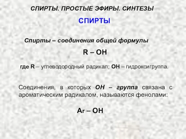 СПИРТЫ