- Lectures ML (3)

Содержание
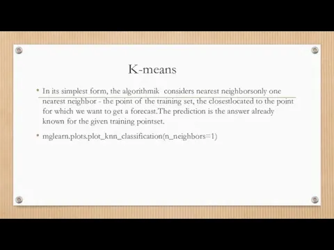
- 2. K-means In its simplest form, the algorithmik considers nearest neighborsonly one nearest neighbor - the point
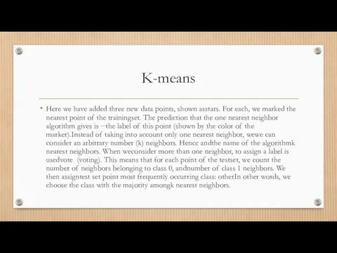
- 3. K-means Here we have added three new data points, shown asstars. For each, we marked the
- 4. K-means In[11]: mglearn.plots.plot_knn_classification(n_neighbors=3)
- 5. K-means and scikit learn Now let's see how the algorithm can be appliedk nearest neighbors using
- 6. K-means and scikit learn Next, we import and create an instance object of the class by
- 7. K-means and sklearn We then fit the classifier using the training set. ForKNeighborsClassifier which means remembering
- 8. Predict To get the predictions for the test data, we call the methodpredict. For each point
- 9. Score In[16]: print("Правильность на тестовом наборе: {:.2f}".format(clf.score(X_test, y_test))) Out[16]: Правильность на тестовом наборе: 0.86
- 10. Boundaries Also, for two-dimensional datasets, we can showpredictions for all possible test set points by placing
- 11. Boundaries In[17]: fig, axes = plt.subplots(1, 3, figsize=(10, 3)) for n_neighbors, ax in zip([1, 3, 9],
- 12. KNeighborsRegressor With regard to our one-dimensional data array, we cansee predictions for all possible feature values
- 13. Code fig, axes = plt.subplots(1, 3, figsize=(15, 4)) # создаем 1000 точек данных, равномерно распределенных между
- 14. Code ax.set_title( "{} neighbor(s)\n train score: {:.2f} test score: {:.2f}".format( n_neighbors, reg.score(X_train, y_train), reg.score(X_test, y_test))) ax.set_xlabel("Признак")
- 15. Advantages and disadvantages Basically, there are two important parameters in the KNeighbors classifier:the number of neighbors
- 16. Advantages and disadvantages Typically, building a modelnearest neighbors happens very fast, but when your trainingthe set
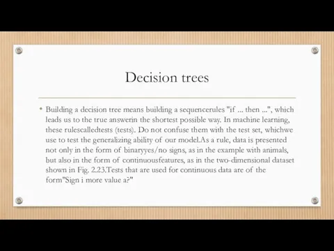
- 17. Decision trees Building a decision tree means building a sequencerules "if ... then ...", which leads
- 18. Decision trees mglearn.plots.plot_tree_progressive()
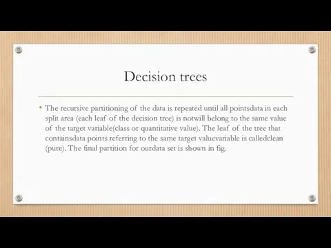
- 19. Decision trees The recursive partitioning of the data is repeated until all pointsdata in each split
- 20. Pruning Let's take a closer look at how preflight works.clipping on the example of the Breast
- 21. Pruning In[58]: from sklearn.tree import DecisionTreeClassifier cancer = load_breast_cancer() X_train, X_test, y_train, y_test = train_test_split( cancer.data,
- 22. Pruning If you do not limit the depth, the tree can be arbitrarilydeep and complex. Therefore,
- 23. Pruning In[59]: tree = DecisionTreeClassifier(max_depth=4, random_state=0) tree.fit(X_train, y_train) print("Правильность на обучающем наборе: {:.3f}".format(tree.score(X_train, y_train))) print("Правильность на
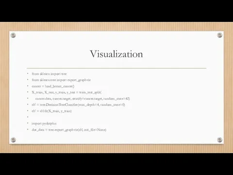
- 24. Visualization from sklearn.tree import export_graphviz export_graphviz(tree, out_file="tree.dot", class_names=["malignant", "benign"], feature_names=cancer.feature_names, impurity=False, filled=True)
- 25. Visualization import graphviz with open("tree.dot") as f: dot_graph = f.read() graphviz.Source(dot_graph)
- 26. Visualization import numpy as np import matplotlib.pyplot as plt import pandas as pd import mglearn %matplotlib
- 27. Visualization from sklearn import tree from sklearn.tree import export_graphviz cancer = load_breast_cancer() X_train, X_test, y_train, y_test
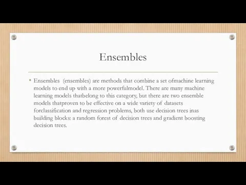
- 28. Ensembles Ensembles (ensembles) are methods that combine a set ofmachine learning models to end up with
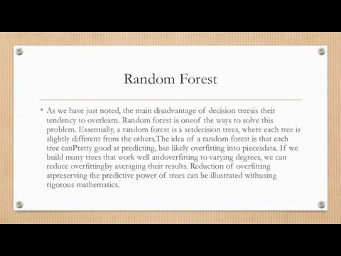
- 29. Random Forest As we have just noted, the main disadvantage of decision treesis their tendency to
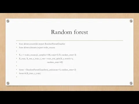
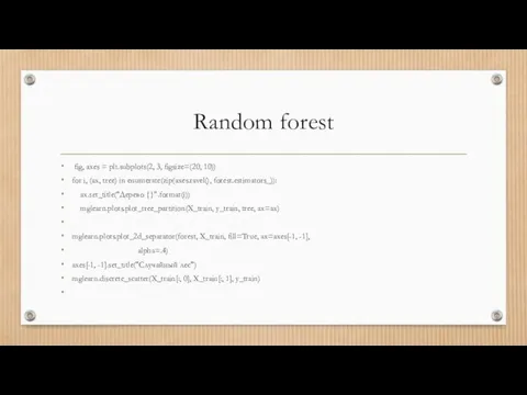
- 30. Random forest from sklearn.ensemble import RandomForestClassifier from sklearn.datasets import make_moons X, y = make_moons(n_samples=100, noise=0.25, random_state=3)
- 31. Random forest fig, axes = plt.subplots(2, 3, figsize=(20, 10)) for i, (ax, tree) in enumerate(zip(axes.ravel(), forest.estimators_)):
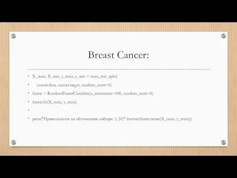
- 32. Breast Cancer: X_train, X_test, y_train, y_test = train_test_split( cancer.data, cancer.target, random_state=0) forest = RandomForestClassifier(n_estimators=100, random_state=0) forest.fit(X_train,
- 33. Breast Cancer: def plot_feature_importances_cancer(model): n_features = cancer.data.shape[1] plt.barh(range(n_features), model.feature_importances_, align='center') plt.yticks(np.arange(n_features), cancer.feature_names) plt.xlabel("Важность признака") plt.ylabel("Признак") plot_feature_importances_cancer(forest)
- 34. Gradient Boosting The basic idea of gradient boosting is to combineset of simple models (in this
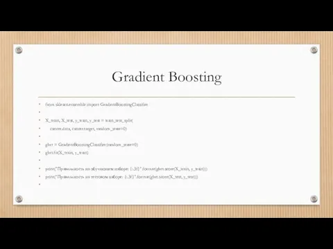
- 35. Gradient Boosting from sklearn.ensemble import GradientBoostingClassifier X_train, X_test, y_train, y_test = train_test_split( cancer.data, cancer.target, random_state=0) gbrt
- 36. Gradient Boosting gbrt = GradientBoostingClassifier(random_state=0, max_depth=1) gbrt.fit(X_train, y_train) print("Правильность на обучающем наборе: {:.3f}".format(gbrt.score(X_train, y_train))) print("Правильность на
- 38. Скачать презентацию
Слайд 2K-means
In its simplest form, the algorithmik considers nearest neighborsonly one nearest neighbor
K-means
In its simplest form, the algorithmik considers nearest neighborsonly one nearest neighbor
Слайд 3K-means
Here we have added three new data points, shown asstars. For each,
K-means
Here we have added three new data points, shown asstars. For each,
Слайд 4K-means
In[11]:
mglearn.plots.plot_knn_classification(n_neighbors=3)
K-means
In[11]:
mglearn.plots.plot_knn_classification(n_neighbors=3)
![K-means In[11]: mglearn.plots.plot_knn_classification(n_neighbors=3)](/_ipx/f_webp&q_80&fit_contain&s_1440x1080/imagesDir/jpg/887732/slide-3.jpg)
Слайд 5K-means and scikit learn
Now let's see how the algorithm can be appliedk
K-means and scikit learn
Now let's see how the algorithm can be appliedk
Слайд 6K-means and scikit learn
Next, we import and create an instance object of
K-means and scikit learn
Next, we import and create an instance object of
Слайд 7K-means and sklearn
We then fit the classifier using the training set. ForKNeighborsClassifier
K-means and sklearn
We then fit the classifier using the training set. ForKNeighborsClassifier
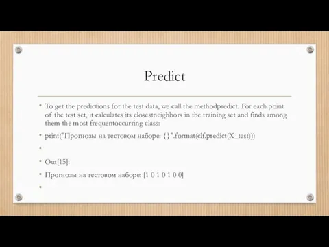
Слайд 8Predict
To get the predictions for the test data, we call the methodpredict.
Predict
To get the predictions for the test data, we call the methodpredict.
Слайд 9Score
In[16]:
print("Правильность на тестовом наборе: {:.2f}".format(clf.score(X_test, y_test)))
Out[16]:
Правильность на тестовом наборе:
Score
In[16]:
print("Правильность на тестовом наборе: {:.2f}".format(clf.score(X_test, y_test)))
Out[16]:
Правильность на тестовом наборе:
![Score In[16]: print("Правильность на тестовом наборе: {:.2f}".format(clf.score(X_test, y_test))) Out[16]: Правильность на тестовом наборе: 0.86](/_ipx/f_webp&q_80&fit_contain&s_1440x1080/imagesDir/jpg/887732/slide-8.jpg)
Слайд 10Boundaries
Also, for two-dimensional datasets, we can showpredictions for all possible test set
Boundaries
Also, for two-dimensional datasets, we can showpredictions for all possible test set

Слайд 11Boundaries
In[17]:
fig, axes = plt.subplots(1, 3, figsize=(10, 3))
for n_neighbors, ax in
Boundaries
In[17]:
fig, axes = plt.subplots(1, 3, figsize=(10, 3))
for n_neighbors, ax in
![Boundaries In[17]: fig, axes = plt.subplots(1, 3, figsize=(10, 3)) for n_neighbors, ax](/_ipx/f_webp&q_80&fit_contain&s_1440x1080/imagesDir/jpg/887732/slide-10.jpg)
Слайд 12KNeighborsRegressor
With regard to our one-dimensional data array, we cansee predictions for all
KNeighborsRegressor
With regard to our one-dimensional data array, we cansee predictions for all
Слайд 13Code
fig, axes = plt.subplots(1, 3, figsize=(15, 4))
# создаем 1000 точек данных,
Code
fig, axes = plt.subplots(1, 3, figsize=(15, 4))
# создаем 1000 точек данных,
Слайд 14Code
ax.set_title(
"{} neighbor(s)\n train score: {:.2f} test score: {:.2f}".format(
n_neighbors,
Code
ax.set_title(
"{} neighbor(s)\n train score: {:.2f} test score: {:.2f}".format(
n_neighbors,
Слайд 15Advantages and disadvantages
Basically, there are two important parameters in the KNeighbors classifier:the
Advantages and disadvantages
Basically, there are two important parameters in the KNeighbors classifier:the

Слайд 16Advantages and disadvantages
Typically, building a modelnearest neighbors happens very fast, but when
Advantages and disadvantages
Typically, building a modelnearest neighbors happens very fast, but when

Слайд 17Decision trees
Building a decision tree means building a sequencerules "if ... then
Decision trees
Building a decision tree means building a sequencerules "if ... then
Слайд 18Decision trees
mglearn.plots.plot_tree_progressive()
Decision trees
mglearn.plots.plot_tree_progressive()
Слайд 19Decision trees
The recursive partitioning of the data is repeated until all pointsdata
Decision trees
The recursive partitioning of the data is repeated until all pointsdata
Слайд 20
Pruning
Let's take a closer look at how preflight works.clipping on the example
Pruning
Let's take a closer look at how preflight works.clipping on the example
Слайд 21Pruning
In[58]:
from sklearn.tree import DecisionTreeClassifier
cancer = load_breast_cancer()
X_train, X_test, y_train, y_test
Pruning
In[58]:
from sklearn.tree import DecisionTreeClassifier
cancer = load_breast_cancer()
X_train, X_test, y_train, y_test
![Pruning In[58]: from sklearn.tree import DecisionTreeClassifier cancer = load_breast_cancer() X_train, X_test, y_train,](/_ipx/f_webp&q_80&fit_contain&s_1440x1080/imagesDir/jpg/887732/slide-20.jpg)
Слайд 22Pruning
If you do not limit the depth, the tree can be arbitrarilydeep
Pruning
If you do not limit the depth, the tree can be arbitrarilydeep
Слайд 23Pruning
In[59]:
tree = DecisionTreeClassifier(max_depth=4, random_state=0)
tree.fit(X_train, y_train)
print("Правильность на обучающем наборе: {:.3f}".format(tree.score(X_train,
Pruning
In[59]:
tree = DecisionTreeClassifier(max_depth=4, random_state=0)
tree.fit(X_train, y_train)
print("Правильность на обучающем наборе: {:.3f}".format(tree.score(X_train,
![Pruning In[59]: tree = DecisionTreeClassifier(max_depth=4, random_state=0) tree.fit(X_train, y_train) print("Правильность на обучающем наборе:](/_ipx/f_webp&q_80&fit_contain&s_1440x1080/imagesDir/jpg/887732/slide-22.jpg)
Слайд 24Visualization
from sklearn.tree import export_graphviz
export_graphviz(tree, out_file="tree.dot", class_names=["malignant", "benign"],
feature_names=cancer.feature_names, impurity=False, filled=True)
Visualization
from sklearn.tree import export_graphviz
export_graphviz(tree, out_file="tree.dot", class_names=["malignant", "benign"],
feature_names=cancer.feature_names, impurity=False, filled=True)
![Visualization from sklearn.tree import export_graphviz export_graphviz(tree, out_file="tree.dot", class_names=["malignant", "benign"], feature_names=cancer.feature_names, impurity=False, filled=True)](/_ipx/f_webp&q_80&fit_contain&s_1440x1080/imagesDir/jpg/887732/slide-23.jpg)
Слайд 25Visualization
import graphviz
with open("tree.dot") as f:
dot_graph = f.read()
graphviz.Source(dot_graph)
Visualization
import graphviz
with open("tree.dot") as f:
dot_graph = f.read()
graphviz.Source(dot_graph)
Слайд 26Visualization
import numpy as np
import matplotlib.pyplot as plt
import pandas as pd
Visualization
import numpy as np
import matplotlib.pyplot as plt
import pandas as pd
Слайд 27Visualization
from sklearn import tree
from sklearn.tree import export_graphviz
cancer = load_breast_cancer()
X_train,
Visualization
from sklearn import tree
from sklearn.tree import export_graphviz
cancer = load_breast_cancer()
X_train,
Слайд 28Ensembles
Ensembles (ensembles) are methods that combine a set ofmachine learning models to
Ensembles
Ensembles (ensembles) are methods that combine a set ofmachine learning models to
Слайд 29Random Forest
As we have just noted, the main disadvantage of decision treesis
Random Forest
As we have just noted, the main disadvantage of decision treesis
Слайд 30Random forest
from sklearn.ensemble import RandomForestClassifier
from sklearn.datasets import make_moons
X, y =
Random forest
from sklearn.ensemble import RandomForestClassifier
from sklearn.datasets import make_moons
X, y =
Слайд 31Random forest
fig, axes = plt.subplots(2, 3, figsize=(20, 10))
for i, (ax,
Random forest
fig, axes = plt.subplots(2, 3, figsize=(20, 10))
for i, (ax,
Слайд 32Breast Cancer:
X_train, X_test, y_train, y_test = train_test_split(
cancer.data, cancer.target, random_state=0)
Breast Cancer:
X_train, X_test, y_train, y_test = train_test_split(
cancer.data, cancer.target, random_state=0)
Слайд 33Breast Cancer:
def plot_feature_importances_cancer(model):
n_features = cancer.data.shape[1]
plt.barh(range(n_features), model.feature_importances_, align='center')
Breast Cancer:
def plot_feature_importances_cancer(model):
n_features = cancer.data.shape[1]
plt.barh(range(n_features), model.feature_importances_, align='center')
![Breast Cancer: def plot_feature_importances_cancer(model): n_features = cancer.data.shape[1] plt.barh(range(n_features), model.feature_importances_, align='center') plt.yticks(np.arange(n_features), cancer.feature_names) plt.xlabel("Важность признака") plt.ylabel("Признак") plot_feature_importances_cancer(forest)](/_ipx/f_webp&q_80&fit_contain&s_1440x1080/imagesDir/jpg/887732/slide-32.jpg)
Слайд 34Gradient Boosting
The basic idea of gradient boosting is to combineset of simple
Gradient Boosting
The basic idea of gradient boosting is to combineset of simple
Слайд 35Gradient Boosting
from sklearn.ensemble import GradientBoostingClassifier
X_train, X_test, y_train, y_test = train_test_split(
Gradient Boosting
from sklearn.ensemble import GradientBoostingClassifier
X_train, X_test, y_train, y_test = train_test_split(
Слайд 36Gradient Boosting
gbrt = GradientBoostingClassifier(random_state=0, max_depth=1)
gbrt.fit(X_train, y_train)
print("Правильность на обучающем наборе: {:.3f}".format(gbrt.score(X_train,
Gradient Boosting
gbrt = GradientBoostingClassifier(random_state=0, max_depth=1)
gbrt.fit(X_train, y_train)
print("Правильность на обучающем наборе: {:.3f}".format(gbrt.score(X_train,
 Презентация на тему Водяной пар Влажность воздуха
 Интерактивные вебинары как новая форма учебной деятельности http://webinar.ffl.msu.ru
 Математический турнир
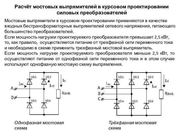 Расчёт мостовых выпрямителей в курсовом проектировании силовых преобразователей
 A day in London
 Приоритетный национальный проект "ОБРАЗОВАНИЕ"
 Преобразование внутреннего школьного пространства
 What language do dolphins speak?
 Аминокислоты Модели молекул
 Сущность аттестации персонала. Проведение аттестации
 Циклотимный тип личности
 Дикое поле 1992
 Базовый курс работы с кожей. Пошив сумок и одежды
 Презентация на тему Основные периоды формирования политической карты мира
 Быть в 10 раз эффективнее благодаря Groovy
 ПОВЫШЕНИЕ ЭФФЕКТИВНОСТИ ПЕРЕРАБОТКИ ВАНАДИЕВОГО ЧУГУНА НА НТМК
 Рисование диких кошек
 Политические партии
 Презентация на тему Алгоритмы сжатия. Алгоритм построения орграфа Хаффмана
 Презентация на тему Начало распада Древнерусского государства
  Былина – эпическая форма фольклора
 Перспективы развития платежной системы Банка России в свете Федерального закона «О национальной платежной системе»
 План проведения педагогического совета 1. Вступление. Анализ выполнения решений предыдущего педагогического совета. 2. Доклад «Сти
 Презентация на тему Пастернак Доктор Живаго
  поговорим о вежливости
 01- System Overview Rev A
 2 часть
 Политическая сфера