- Теория Информации

Содержание
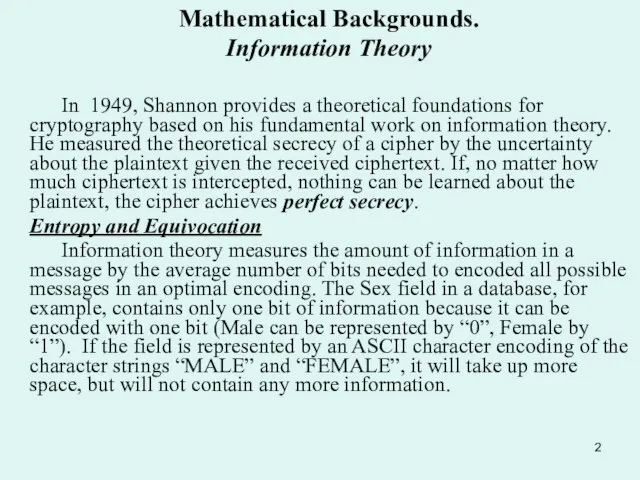
- 2. Mathematical Backgrounds. Information Theory In 1949, Shannon provides a theoretical foundations for cryptography based on his
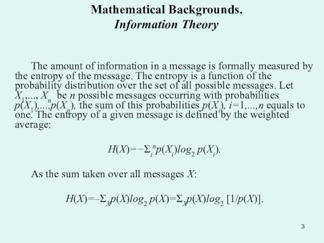
- 3. Mathematical Backgrounds. Information Theory The amount of information in a message is formally measured by the
- 4. Mathematical Backgrounds. Information theory in Examples Intuitively, each term log2 [1/p(X)] in last expression represents the
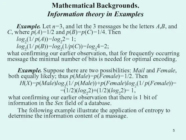
- 5. Mathematical Backgrounds. Information theory in Examples Example. Let n=3, and let the 3 messages be the
- 6. Example. Let n=3, and let the 3 messages be the letter A,B,and C, where p(A)=1/2, p(B)=p(C)=1/4.
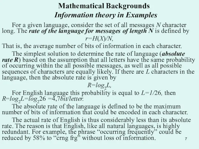
- 7. Mathematical Backgrounds Information theory in Examples For a given language, consider the set of all messages
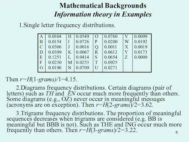
- 8. Mathematical Backgrounds Information theory in Examples 1.Single letter frequency distributions. Then r=H(1-grams)/1=4.15. 2.Diagrams frequency distributions. Certain
- 9. The rate of a language (entropy per character) is determined by estimating the entropy of N-grams
- 10. Mathematical Backgrounds Perfect Secrecy Shannon studied the information theoretic properties of cryptographic systems in terms of
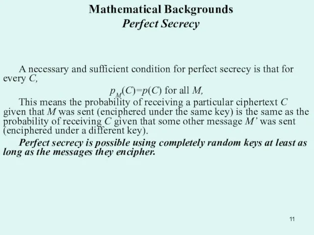
- 11. Mathematical Backgrounds Perfect Secrecy A necessary and sufficient condition for perfect secrecy is that for every
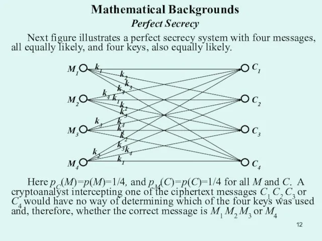
- 12. Mathematical Backgrounds Perfect Secrecy Next figure illustrates a perfect secrecy system with four messages, all equally
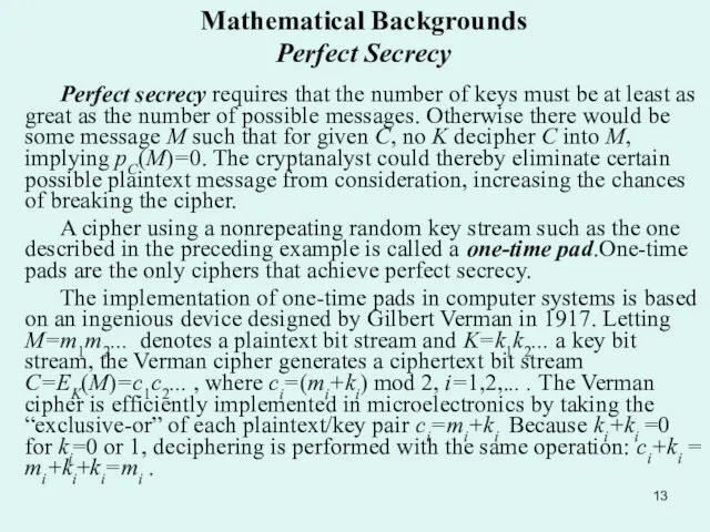
- 13. Mathematical Backgrounds Perfect Secrecy Perfect secrecy requires that the number of keys must be at least
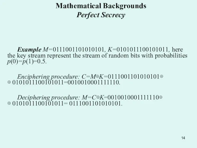
- 14. Mathematical Backgrounds Perfect Secrecy Example M=0111001101010101, K=0101011100101011, here the key stream represent the stream of random
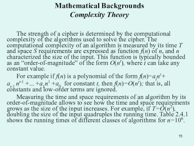
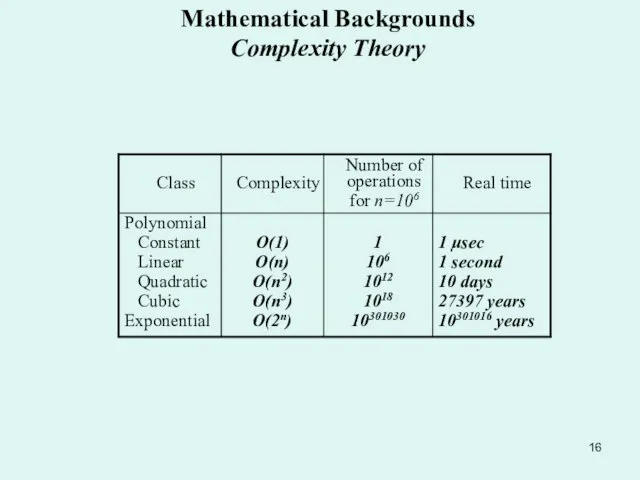
- 15. Mathematical Backgrounds Complexity Theory The strength of a cipher is determined by the computational complexity of
- 16. Mathematical Backgrounds Complexity Theory
- 17. Mathematical Backgrounds Complexity Theory Complexity theory classifies a problem according to the minimum time and space
- 19. Скачать презентацию
Слайд 2Mathematical Backgrounds.
Information Theory
In 1949, Shannon provides a theoretical foundations for cryptography
Mathematical Backgrounds.
Information Theory
In 1949, Shannon provides a theoretical foundations for cryptography
Слайд 3Mathematical Backgrounds.
Information Theory
The amount of information in a message is formally
Mathematical Backgrounds.
Information Theory
The amount of information in a message is formally
Слайд 4Mathematical Backgrounds.
Information theory in Examples
Intuitively, each term log2 [1/p(X)] in last
Mathematical Backgrounds.
Information theory in Examples
Intuitively, each term log2 [1/p(X)] in last
![Mathematical Backgrounds. Information theory in Examples Intuitively, each term log2 [1/p(X)] in](/_ipx/f_webp&q_80&fit_contain&s_1440x1080/imagesDir/jpg/376023/slide-3.jpg)
Слайд 5Mathematical Backgrounds.
Information theory in Examples
Example. Let n=3, and let the 3
Mathematical Backgrounds.
Information theory in Examples
Example. Let n=3, and let the 3
Слайд 6
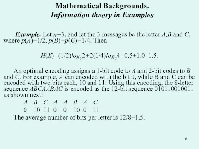
Example. Let n=3, and let the 3 messages be the letter
Example. Let n=3, and let the 3 messages be the letter
Слайд 7Mathematical Backgrounds
Information theory in Examples
For a given language, consider the
Mathematical Backgrounds
Information theory in Examples
For a given language, consider the
Слайд 8Mathematical Backgrounds
Information theory in Examples
1.Single letter frequency distributions.
Then r=H(1-grams)/1=4.15.
2.Diagrams frequency
Mathematical Backgrounds
Information theory in Examples
1.Single letter frequency distributions.
Then r=H(1-grams)/1=4.15.
2.Diagrams frequency
Слайд 9 The rate of a language (entropy per character) is determined by estimating
The rate of a language (entropy per character) is determined by estimating
Слайд 10Mathematical Backgrounds Perfect Secrecy
Shannon studied the information theoretic properties of cryptographic
Mathematical Backgrounds Perfect Secrecy
Shannon studied the information theoretic properties of cryptographic
Слайд 11Mathematical Backgrounds Perfect Secrecy
A necessary and sufficient condition for perfect secrecy
Mathematical Backgrounds Perfect Secrecy
A necessary and sufficient condition for perfect secrecy
Слайд 12Mathematical Backgrounds Perfect Secrecy
Next figure illustrates a perfect secrecy system with four
Mathematical Backgrounds Perfect Secrecy
Next figure illustrates a perfect secrecy system with four
Слайд 13Mathematical Backgrounds Perfect Secrecy
Perfect secrecy requires that the number of keys must
Mathematical Backgrounds Perfect Secrecy
Perfect secrecy requires that the number of keys must
Слайд 14Mathematical Backgrounds Perfect Secrecy
Example M=0111001101010101, K=0101011100101011, here the key stream represent the
Mathematical Backgrounds Perfect Secrecy
Example M=0111001101010101, K=0101011100101011, here the key stream represent the
Слайд 15Mathematical Backgrounds Complexity Theory
The strength of a cipher is determined by the
Mathematical Backgrounds Complexity Theory
The strength of a cipher is determined by the
Слайд 16Mathematical Backgrounds Complexity Theory
Mathematical Backgrounds Complexity Theory
Слайд 17Mathematical Backgrounds Complexity Theory
Complexity theory classifies a problem according to the minimum
Mathematical Backgrounds Complexity Theory
Complexity theory classifies a problem according to the minimum
 Муниципальное дошкольное образовательное учреждение «Центр развития ребенка – детский сад № 9» Проект «В поисках лета»
 Изменения в нормативной правовой базе ЕГЭ в 2012 г.
 Работа выполнена в рамках проекта: «Повышение квалификации различных категорий работников образования и формирование у них базов
 Смольный институт благородных девиц
 НАПРАВЛЕНИЯ ДЕЯТЕЛЬНОСТИ ЦЕНТРА ЭКОЛОГИЧЕСКОГО МОНИТОРИНГА И КОММЕРЦИАЛИЗАЦИЯ НАУЧНЫХ ИССЛЕДОВАНИЙ
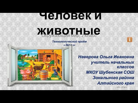 Презентация на тему Человек и животные 2 класс
  ФРАНЦІЯ: ВІД МОНАРХІI ДО РЕСПУБЛІКИ
  20161006_tema_uroka_5_klass_svyaz_muzyki_i_literatury
 Процедура оказания услуги удостоверяющего центра (УЦ). Проверка предоставленных сведений в УЦ
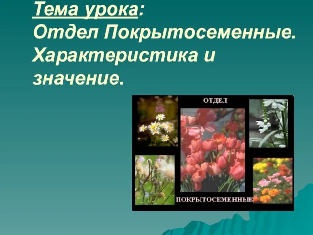 Отдел Покрытосеменные. Характеристика и значение
 Публицистический стиль речи: особенности, жанры, сфера употребления
 הַ יְלָ ִדים רֹוצִ ים ִללמֹוד ִע ְב ִרית בֶּ אּולפַ ן ֶהחָ ָדׁש
 Деловое совещание
 Тема урока: «Знакомство с бытом и жилищем казаков». Подготовила:
  Пунктуация в сложном предложении
 Ростехнадзор. Объект контроля
 Союз Поволжья
 Поздравление с Днем Защитника Отечества
 Презентация на тему НАЧАЛО РАЗДРОБЛЕННОСТИ НА РУСИ
  Презентация на тему Художественная культура Исламского Востока
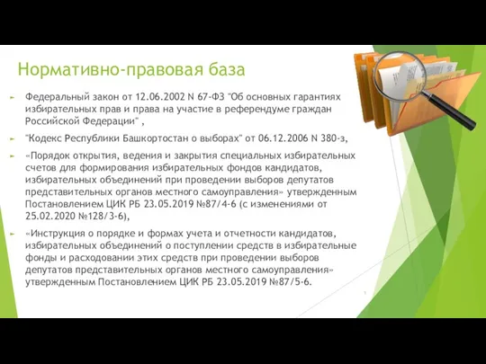 Избирательные фонды кандидатов
 Конференция.
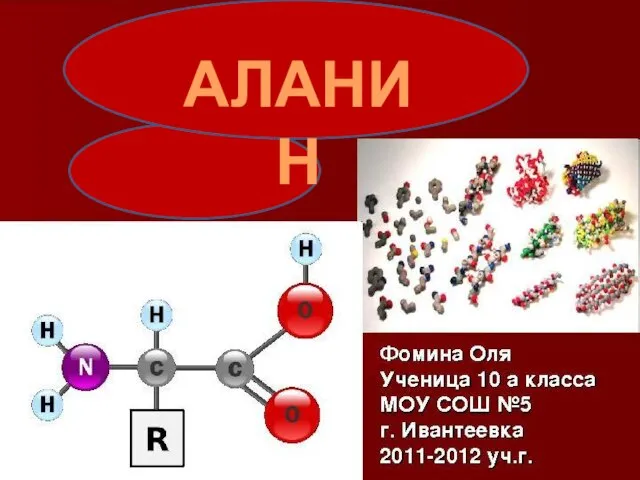 Аланин
 ДОБРО ПОЖАЛОВАТЬ НА ЗАВОД LG ELECTRONICSВ РОССИИ !
 История открытия
 Що я знаю про Power Point
 Твой дом. Твой стиль
 Почвенные ресурсы России 8 класс