- Macroeconomics 7

Содержание
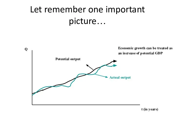
- 2. Let remember one important picture… Potential output Actual output Economic growth can be treated as an
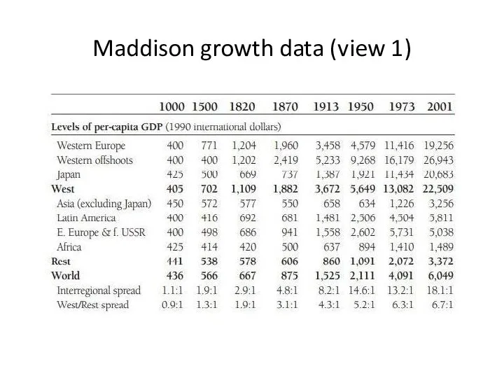
- 3. Maddison growth data (view 1)
- 4. Perhaps, you heard in the introductory course about… hockey stick of economic progress!
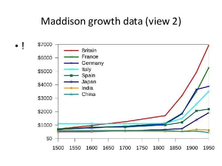
- 5. Maddison growth data (view 2) !
- 6. Economic Theory of the XIX Century: An example of “Outdated” View on Growth – part 1
- 7. Economic Theory of the XIX Century: An example of “Outdated” View on Growth – part 2
- 8. Towards the contemporary theory of growth – part 1 Harrod (1939) and Domar (1946) laid the
- 9. Towards the contemporary theory of growth – part 2 So, Harrod and Domar created the models
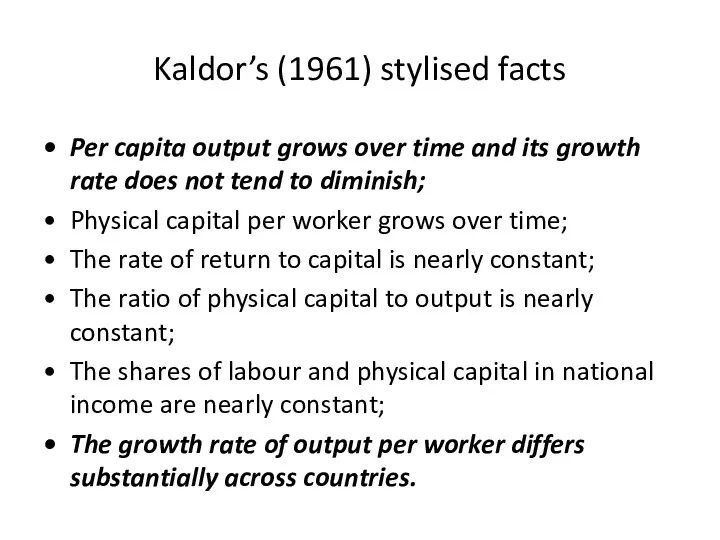
- 10. Kaldor’s (1961) stylised facts Per capita output grows over time and its growth rate does not
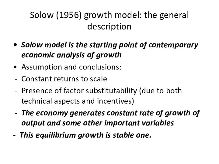
- 11. Solow (1956) growth model: the general description Solow model is the starting point of contemporary economic
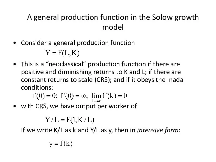
- 12. A general production function in the Solow growth model Consider a general production function This is
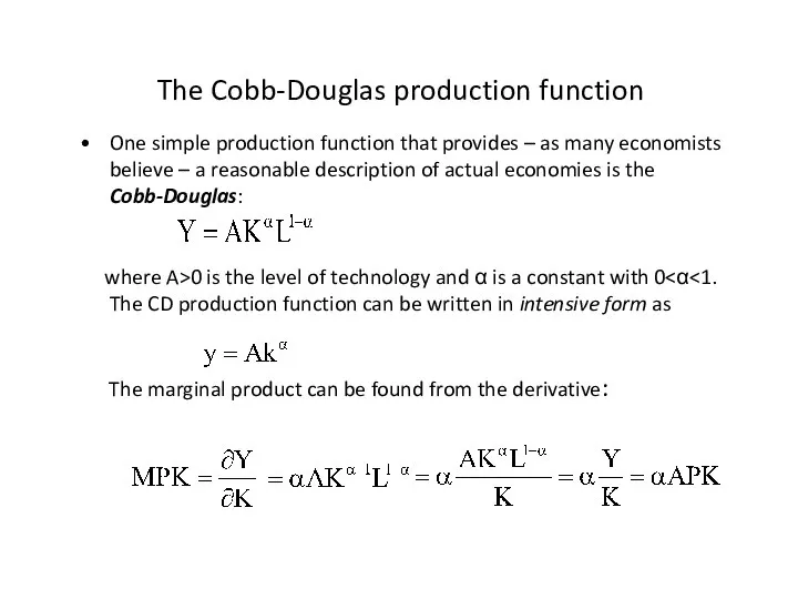
- 13. The Cobb-Douglas production function One simple production function that provides – as many economists believe –
- 14. Results for distribution of income If firms pay workers a wage of w, and pay r
- 15. Diminishing returns to capital output per worker, y=f(k)=kα f(k) k
- 16. The economy is saving and investing a constant fraction of income… gross investment per worker, sf(k)=skα
- 17. What is “labor-augmenting technical progress”? This is technical progress that increases contribution of labor into output!
- 18. If we take into account “labor-augmenting technical progress” that
- 19. Production function with technical progress in the intensive form
- 20. What is break-even investment?
- 21. Derivation of equilibrium capital per effective worker
- 22. Equilibrium as a situation of steady-state growth
- 23. Dynamics of parameters on the steady-state
- 24. Balanced growth
- 25. Growth in steady state and outside steady state In the steady state – when actual investment
- 26. Unconditional convergence
- 27. Conditional convergence
- 28. The concept of the Golden Rule
- 29. The Golden Rule – for what?
- 30. The U.S. Golden Rule – Estimation (Part 1)
- 31. The U.S. Golden Rule – Estimation (Part 2)
- 32. The U.S. Golden Rule – Estimation (Part 3)
- 33. The U.S. Golden Rule – Estimation (Part 4)
- 34. When saving rate is too much high
- 35. Accounting of growth in Solow model (Part 1)
- 36. Accounting of growth in Solow model (Part 2)
- 37. Accounting of growth in Solow model (Part 3)
- 38. Accounting of growth in the U.S. economy In the end of the XX century
- 39. Accounting of growth among “Asian Tigers” In the end of the XX century
- 41. Скачать презентацию
Слайд 2Let remember one important picture…
Potential output
Actual output
Economic growth can be treated as
an
Let remember one important picture…
Potential output
Actual output
Economic growth can be treated as
an
Слайд 3Maddison growth data (view 1)
Maddison growth data (view 1)
Слайд 4Perhaps, you heard in the introductory course about…
hockey stick of economic progress!
Perhaps, you heard in the introductory course about…
hockey stick of economic progress!
Слайд 5Maddison growth data (view 2)
!
Maddison growth data (view 2)
!
Слайд 6Economic Theory of the XIX Century: An example of “Outdated” View on
Economic Theory of the XIX Century: An example of “Outdated” View on
Слайд 7Economic Theory of the XIX Century: An example of “Outdated” View on
Economic Theory of the XIX Century: An example of “Outdated” View on
Слайд 8Towards the contemporary theory of growth – part 1
Harrod (1939) and Domar
Towards the contemporary theory of growth – part 1
Harrod (1939) and Domar
Слайд 9Towards the contemporary theory of growth – part 2
So, Harrod and Domar
Towards the contemporary theory of growth – part 2
So, Harrod and Domar
Слайд 10Kaldor’s (1961) stylised facts
Per capita output grows over time and its growth
Kaldor’s (1961) stylised facts
Per capita output grows over time and its growth
Слайд 11Solow (1956) growth model: the general description
Solow model is the starting point
Solow (1956) growth model: the general description
Solow model is the starting point
Слайд 12A general production function in the Solow growth model
Consider a general production
A general production function in the Solow growth model
Consider a general production
Слайд 13The Cobb-Douglas production function
One simple production function that provides – as many
The Cobb-Douglas production function
One simple production function that provides – as many
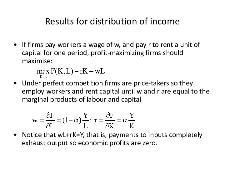
Слайд 14Results for distribution of income
If firms pay workers a wage of w,
Results for distribution of income
If firms pay workers a wage of w,
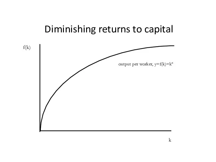
Слайд 15Diminishing returns to capital
output per worker, y=f(k)=kα
f(k)
k
Diminishing returns to capital
output per worker, y=f(k)=kα
f(k)
k
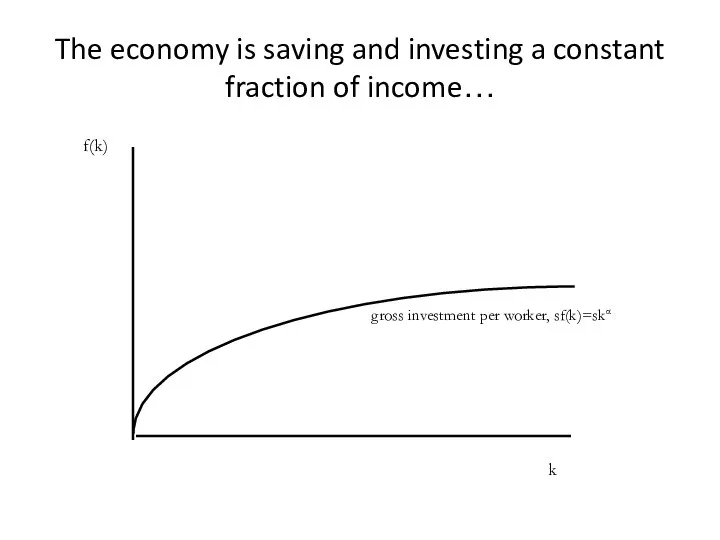
Слайд 16The economy is saving and investing a constant fraction of income…
gross investment
The economy is saving and investing a constant fraction of income…
gross investment
Слайд 17What is “labor-augmenting technical progress”?
This is technical progress that increases contribution of
What is “labor-augmenting technical progress”?
This is technical progress that increases contribution of
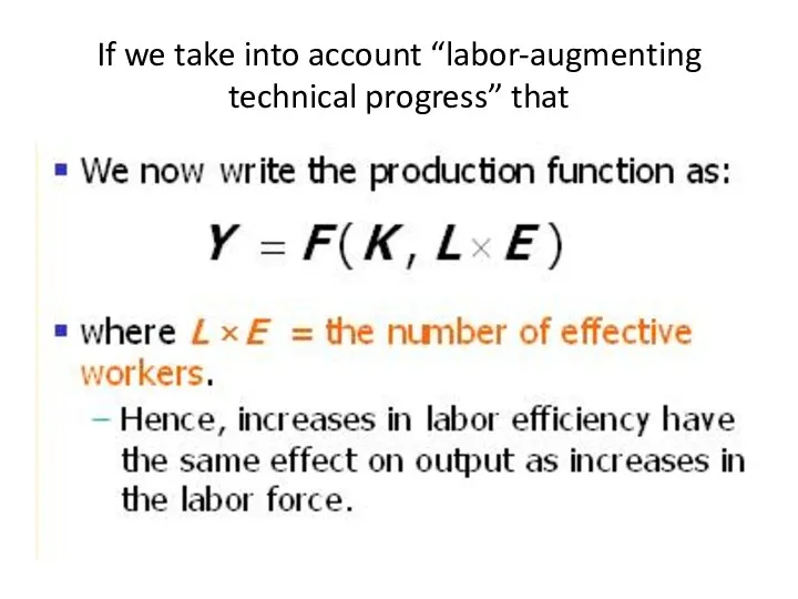
Слайд 18If we take into account “labor-augmenting technical progress” that
If we take into account “labor-augmenting technical progress” that
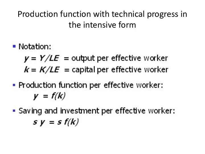
Слайд 19Production function with technical progress in the intensive form
Production function with technical progress in the intensive form
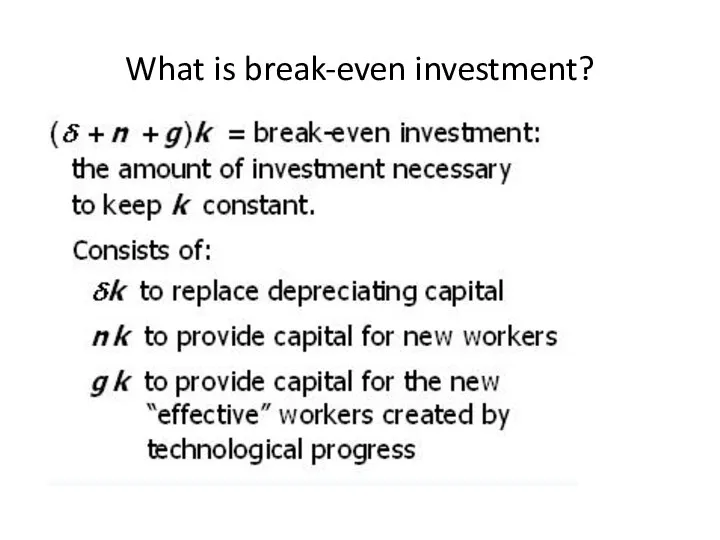
Слайд 20What is break-even investment?
What is break-even investment?
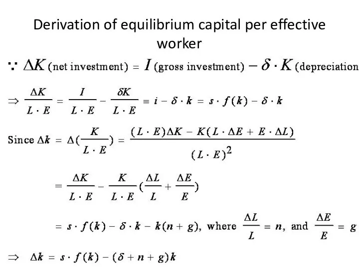
Слайд 21Derivation of equilibrium capital per effective worker
Derivation of equilibrium capital per effective worker
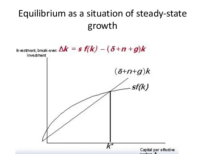
Слайд 22Equilibrium as a situation of steady-state growth
Equilibrium as a situation of steady-state growth
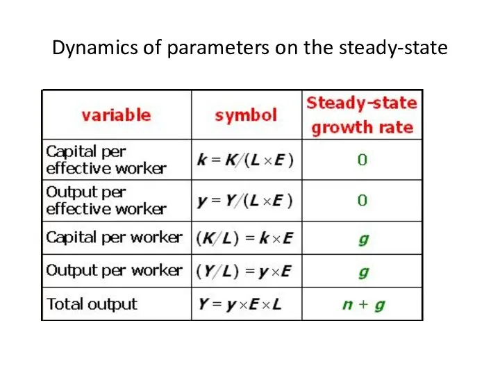
Слайд 23Dynamics of parameters on the steady-state
Dynamics of parameters on the steady-state
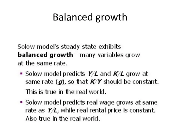
Слайд 24Balanced growth
Balanced growth
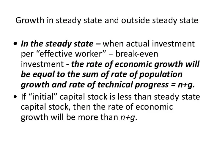
Слайд 25Growth in steady state and outside steady state
In the steady state –
Growth in steady state and outside steady state
In the steady state –
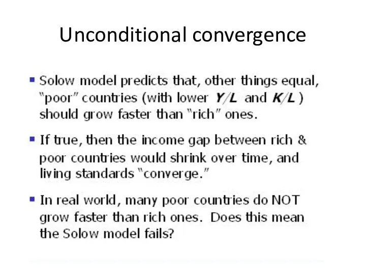
Слайд 26Unconditional convergence
Unconditional convergence
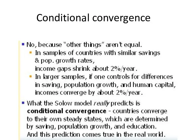
Слайд 27Conditional convergence
Conditional convergence
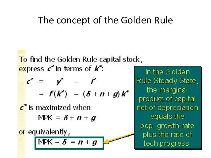
Слайд 28The concept of the Golden Rule
The concept of the Golden Rule
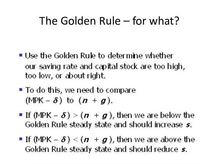
Слайд 29The Golden Rule – for what?
The Golden Rule – for what?
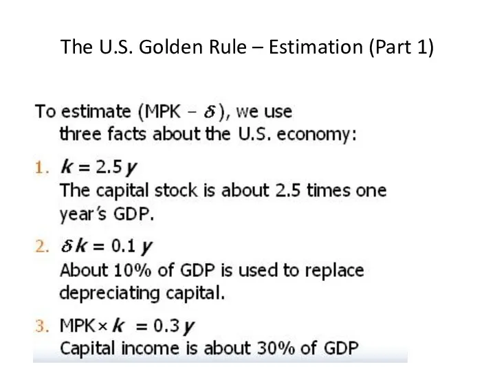
Слайд 30The U.S. Golden Rule – Estimation (Part 1)
The U.S. Golden Rule – Estimation (Part 1)
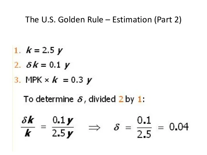
Слайд 31The U.S. Golden Rule – Estimation (Part 2)
The U.S. Golden Rule – Estimation (Part 2)
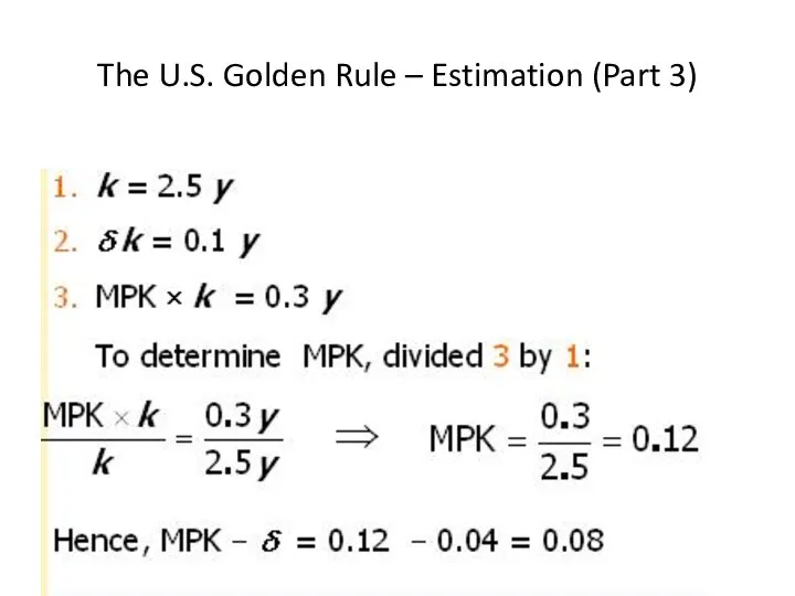
Слайд 32The U.S. Golden Rule – Estimation (Part 3)
The U.S. Golden Rule – Estimation (Part 3)
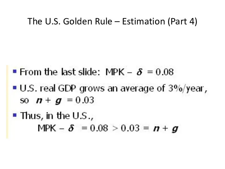
Слайд 33The U.S. Golden Rule – Estimation (Part 4)
The U.S. Golden Rule – Estimation (Part 4)
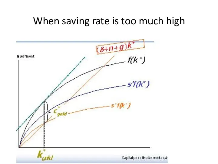
Слайд 34When saving rate is too much high
When saving rate is too much high
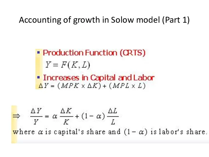
Слайд 35Accounting of growth in Solow model (Part 1)
Accounting of growth in Solow model (Part 1)
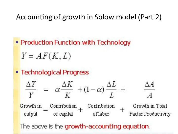
Слайд 36Accounting of growth in Solow model (Part 2)
Accounting of growth in Solow model (Part 2)
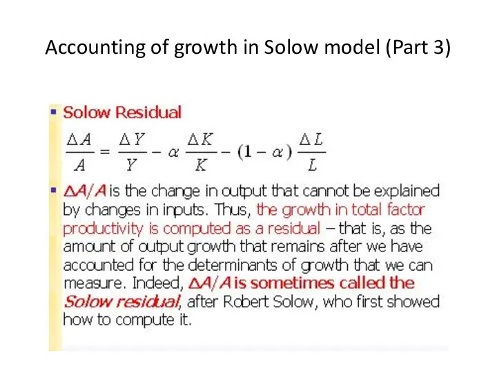
Слайд 37Accounting of growth in Solow model (Part 3)
Accounting of growth in Solow model (Part 3)
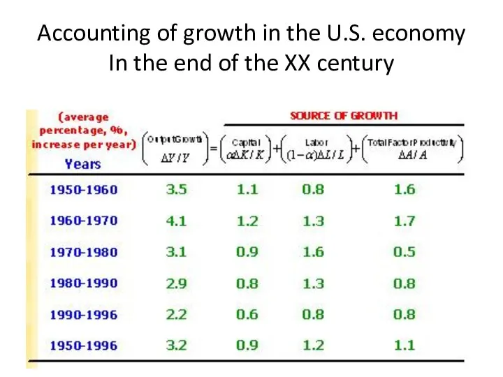
Слайд 38Accounting of growth in the U.S. economy In the end of the
Accounting of growth in the U.S. economy In the end of the
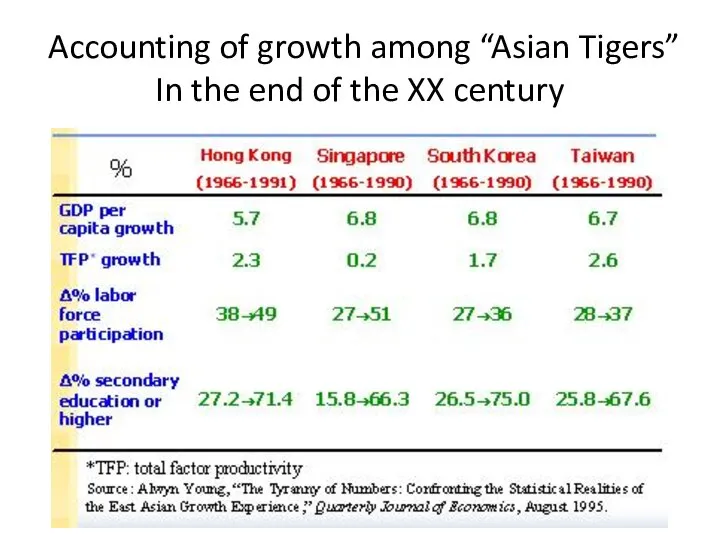
Слайд 39Accounting of growth among “Asian Tigers” In the end of the XX
Accounting of growth among “Asian Tigers” In the end of the XX
 Экономическая теория: предмет и методы, этапы развития. Потребности и ресурсы. Проблема выбора в экономике
 Структура производственного потенциала сельхозпредприятий
 Энергетический дозор
 Особые Экономические Зоны в РФ
 Методы экономической теории
 Понимание различных факторов и их влияние на рынок поставки
 Решение задач по теме: инфляция
 Производство. Тема 5
 Identification de marché et analyse swot
 Эко тимуровцы. Республиканский проект
 Теория «общества кочевников»
 Семейное хозяйство
 Економічна теорія: школи та методи. Тенденції розвитку інформаційного суспільства
 Различные аспекты и методы управления организацией
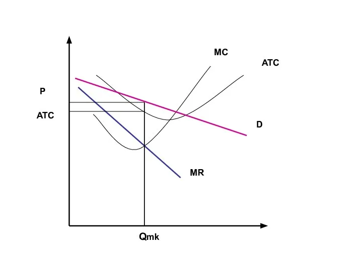 Монополия. Спрос в условиях монополии
 Введение в микроанализ
 Главные вопросы экономики. 9 класс
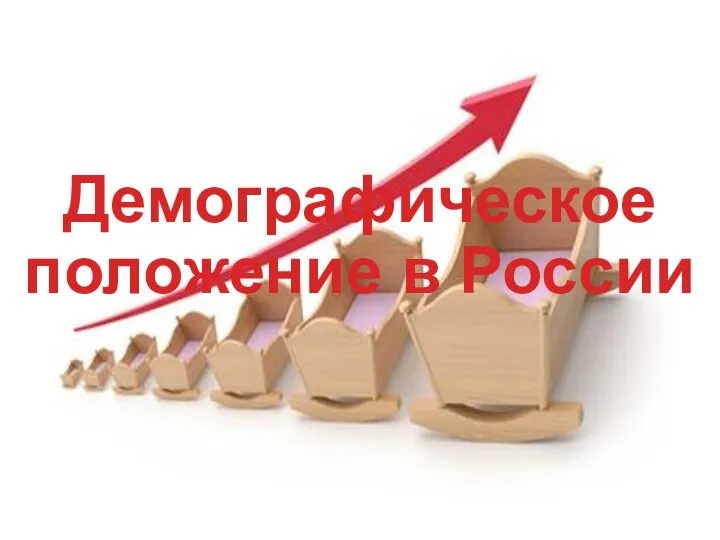 Демографическое положение в России
 Основные итоги внешнеторговой деятельности Астраханской области в 2020 году
 Энергосберегающая политика РФ
 Экономика здравоохранения
 Понятие экономики здравоохранения. Формирование рыночных отношений в здравоохранении. Тема 6
 Суть планируемых изменений в расчете ЗП сотрудников на КТУ+
 Порядок формирования прибыли организации
 Международная торговля товарами и услугами Новой Зеландии и ЮАР Подготовили: Сакович Мария Смыченко Иван Трусова Екатерина Хом
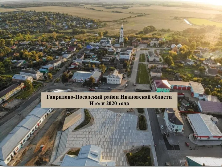 Гаврилово-Посадский район Ивановской области
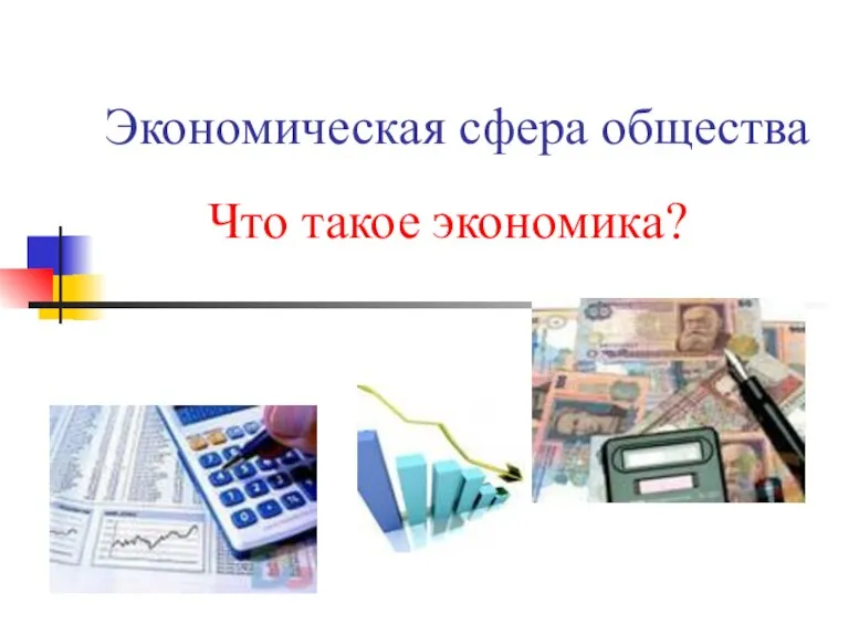 Что такое экономика?
 Август Лёш Теория экономического ландшафта