- Azərbaycan Dövlət Neft və Sənaye Universiteti Optimal Control

Содержание
- 2. Variational Approach to the Fixed-Time, Free-Endpoint Problem
- 3. We now want to see how far a variational approach – i.e. an approach based on
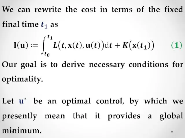
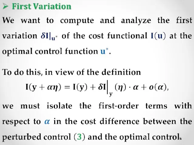
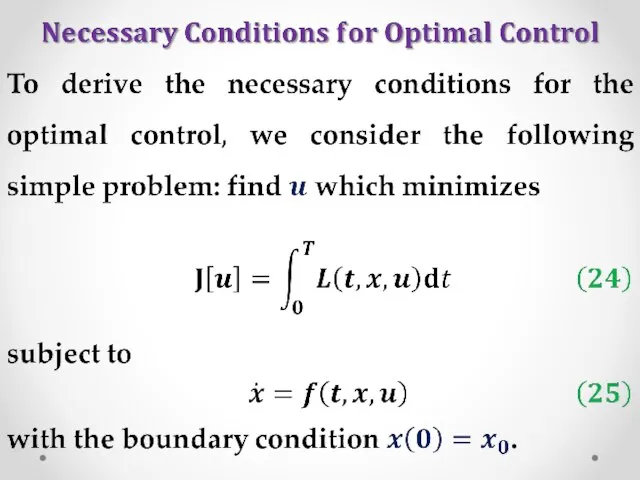
- 6. Our goal is to derive necessary conditions for optimality.
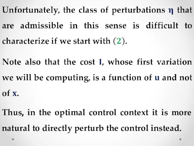
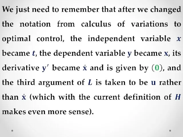
- 8. Thus, in the optimal control context it is more natural to directly perturb the control instead.
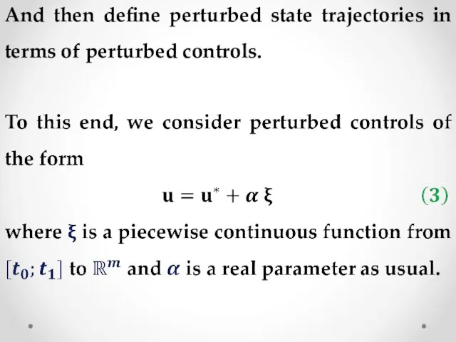
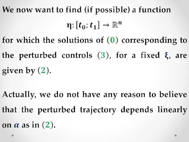
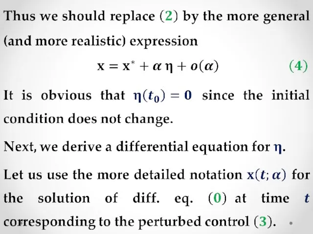
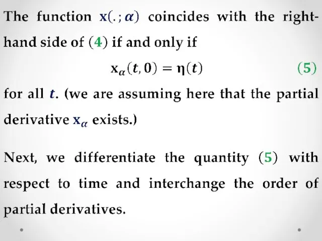
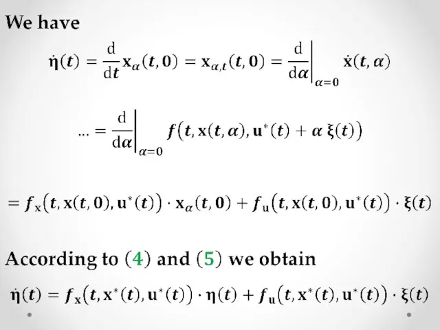
- 9. And then define perturbed state trajectories in terms of perturbed controls.
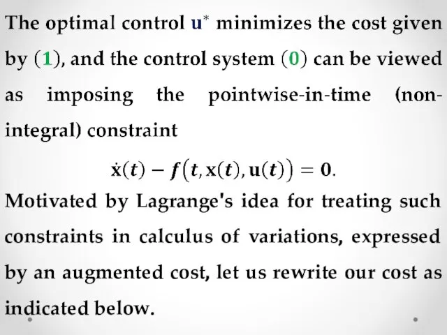
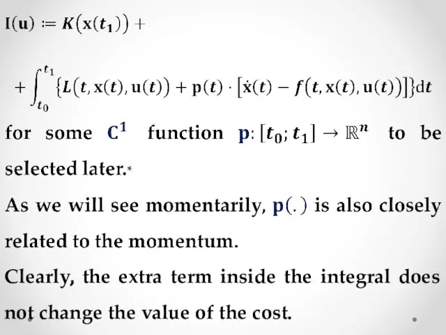
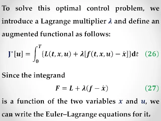
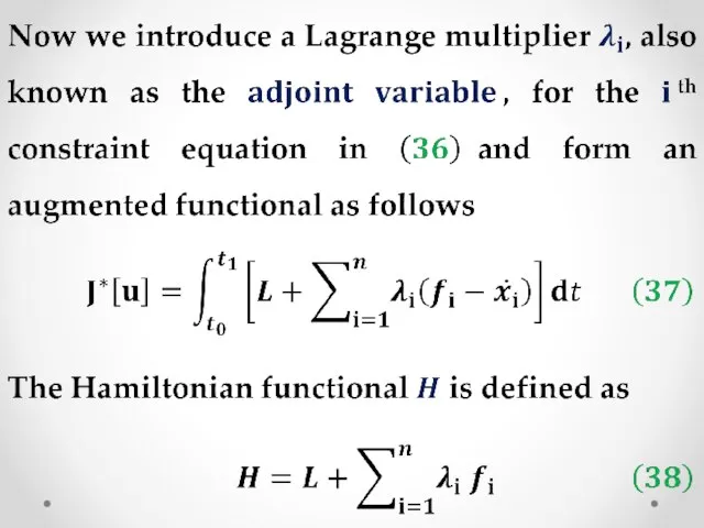
- 16. Motivated by Lagrange's idea for treating such constraints in calculus of variations, expressed by an augmented
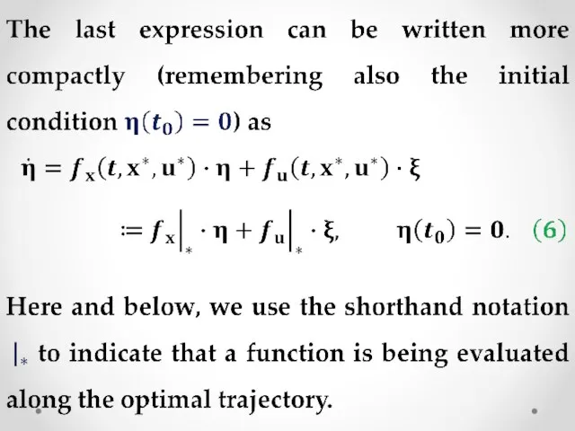
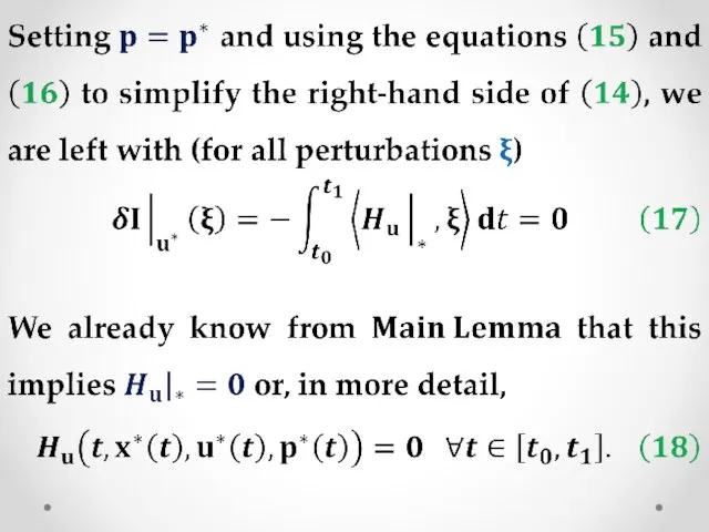
- 17. Clearly, the extra term inside the integral does not change the value of the cost.
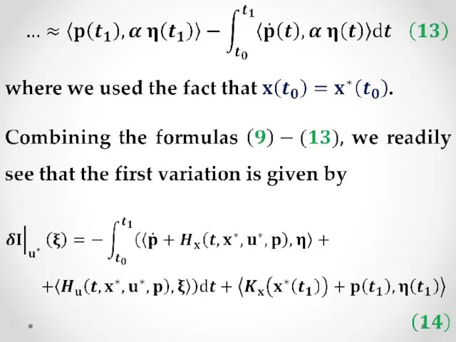
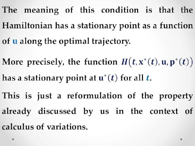
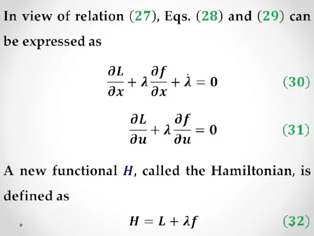
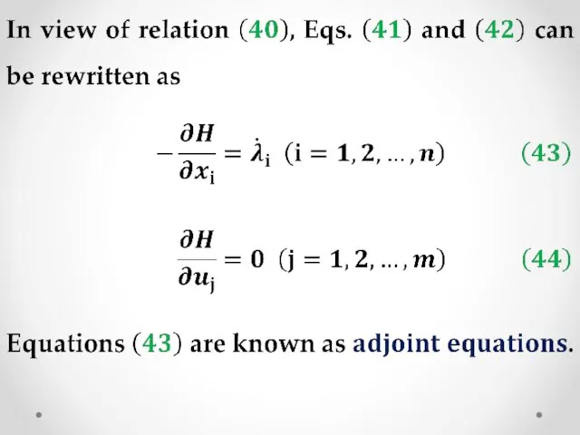
- 31. This is just a reformulation of the property already discussed by us in the context of
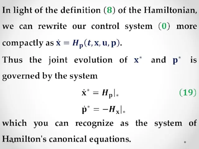
- 32. which you can recognize as the system of Hamilton's canonical equations.
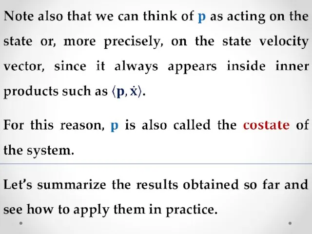
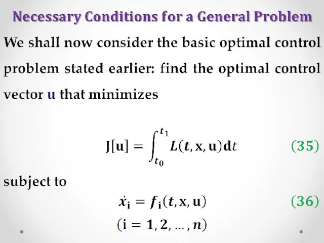
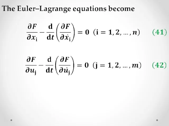
- 35. Let’s summarize the results obtained so far and see how to apply them in practice.
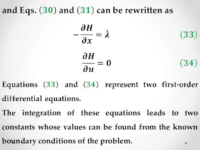
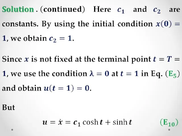
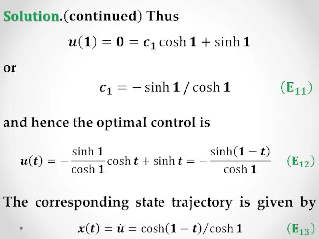
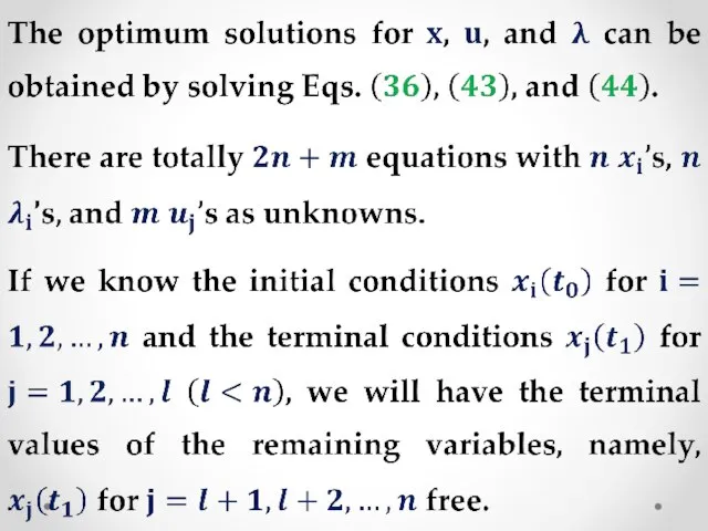
- 43. The integration of these equations leads to two constants whose values can be found from the
- 60. Thank you for attention
- 62. Скачать презентацию
Слайд 3We now want to see how far a variational approach – i.e.
We now want to see how far a variational approach – i.e.
Слайд 6
Our goal is to derive necessary conditions for optimality.
Our goal is to derive necessary conditions for optimality.
Слайд 8
Thus, in the optimal control context it is more natural to directly
Thus, in the optimal control context it is more natural to directly
Слайд 9And then define perturbed state trajectories in terms of perturbed controls.
And then define perturbed state trajectories in terms of perturbed controls.
Слайд 16
Motivated by Lagrange's idea for treating such constraints in calculus of variations,
Motivated by Lagrange's idea for treating such constraints in calculus of variations,
Слайд 17Clearly, the extra term inside the integral does not change the value
Clearly, the extra term inside the integral does not change the value
Слайд 31
This is just a reformulation of the property already discussed by us
This is just a reformulation of the property already discussed by us
Слайд 32
which you can recognize as the system of Hamilton's canonical equations.
which you can recognize as the system of Hamilton's canonical equations.

Слайд 35
Let’s summarize the results obtained so far and see how to apply
Let’s summarize the results obtained so far and see how to apply
Слайд 43
The integration of these equations leads to two constants whose values can
The integration of these equations leads to two constants whose values can


Слайд 60Thank you for attention
Thank you for attention
 Решение теорем
 Корень степени n
 Логарифмы вокруг нас
 Действия с дробями. Нахождение целого по его части и нахождение части целого
 История симметрии
 Формула Ньютона-Лейбница. Площадь криволинейной трапеции
 Справочник по геометрии
 Аксиома параллельных прямых
 Занимательная математика
 Умножение десятичных дробей на натуральные числа
 Маршрут путешествия
 Анализ задач и альтернативные методы решений. Мастер-класс
 Решение тригонометрических уравнений
 В стране математики
 Геометрическая прогрессия в экономике
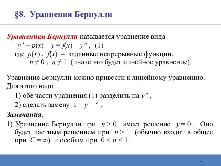 Уравнение Бернулли
 Элементы комбинаторики
 Площадь параллелограмма
 Решение задач на вычисление площадей четырехугольников
 Комбинаторные задачи
 Прямоугольная система координат в пространстве. Координаты вектора
 Элементы высшей математики
 Трапеция. Свойство углов равнобедренной трапеции
 Вычисление площадей плоских фигур. Трапеция
 Формулы приведения
 Принципы статистического оценивания. Анализ данных
 Математика на страницах книг
 Тригонометрические таблицы