- Good morning! Доброе утро! 早上好! Machine learning lecture 3

Содержание
- 2. 我们会成功 We will succeed ! У нас все получится [U nas vse poluchitsya ] ! Без
- 3. . Lecture3. Data preproccessing and machine learning with Scikit-learn
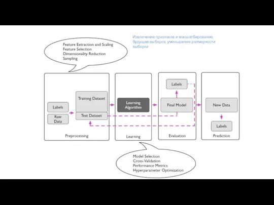
- 4. Извлечение признаков и масшатбирование, будущая выборка, уменьшение размерности выборки
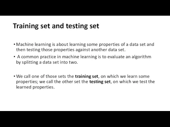
- 5. Training set and testing set Machine learning is about learning some properties of a data set
- 6. Reading a Dataset
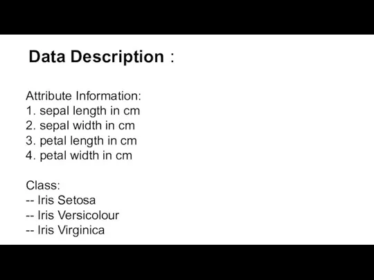
- 8. Data Description : Attribute Information: 1. sepal length in cm 2. sepal width in cm 3.
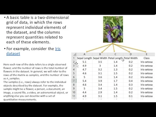
- 9. A basic table is a two-dimensional grid of data, in which the rows represent individual elements
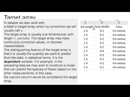
- 10. Target array In dataset we also work with a label or target array, which by convention
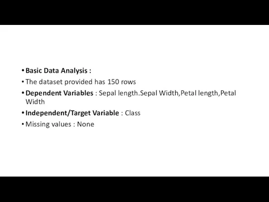
- 11. Basic Data Analysis : The dataset provided has 150 rows Dependent Variables : Sepal length.Sepal Width,Petal
- 12. The dataset is divided into Train and Test data with 80:20 split ratio where 80% data
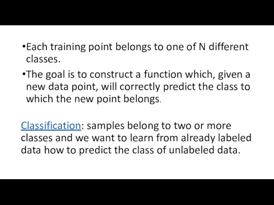
- 13. Each training point belongs to one of N different classes. The goal is to construct a
- 14. What is scikit-learn? The scikit-learn library provides an implementation of a range of algorithms for Supervised
- 15. You can watch the Pandas and scikit-learn features documentation on this site. https://pandas.pydata.org/pandas-docs/stable/ https://scikit-learn.org/stable/documentation.html
- 16. Preprocessing Data: missing data Real world data is filled with missing values. You will often need
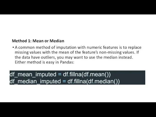
- 18. Method 1: Mean or Median A common method of imputation with numeric features is to replace
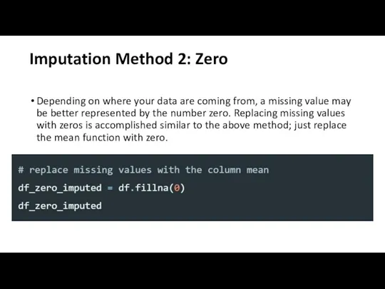
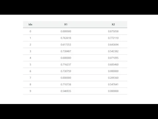
- 20. Imputation Method 2: Zero Depending on where your data are coming from, a missing value may
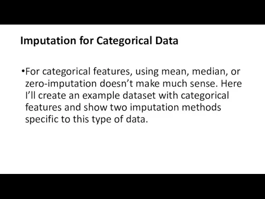
- 22. Imputation for Categorical Data For categorical features, using mean, median, or zero-imputation doesn’t make much sense.
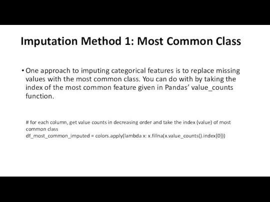
- 24. Imputation Method 1: Most Common Class One approach to imputing categorical features is to replace missing
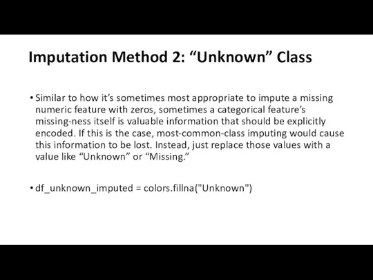
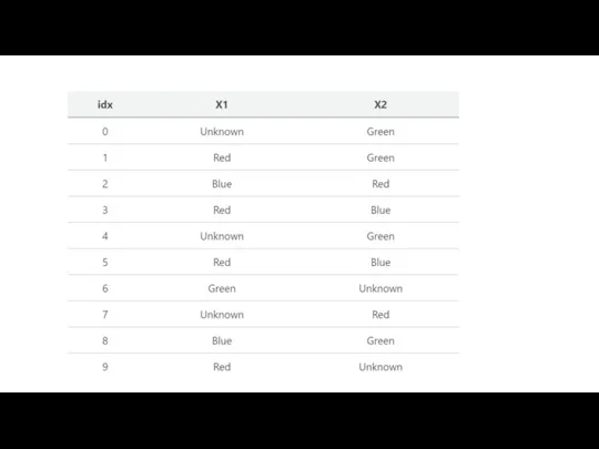
- 26. Imputation Method 2: “Unknown” Class Similar to how it’s sometimes most appropriate to impute a missing
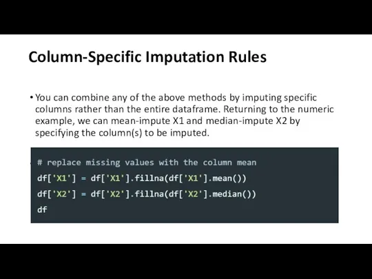
- 28. Column-Specific Imputation Rules You can combine any of the above methods by imputing specific columns rather
- 29. Preprocessing Data If data set are strings We saw in our initial exploration that most of
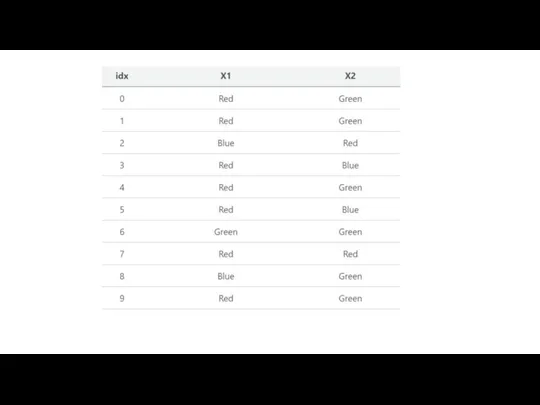
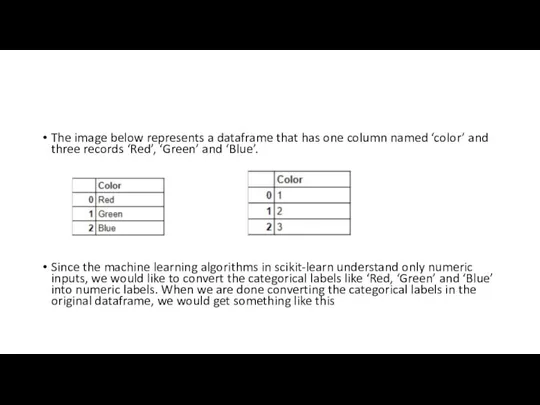
- 30. The image below represents a dataframe that has one column named ‘color’ and three records ‘Red’,
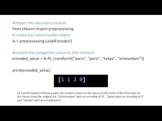
- 31. #import the necessary module from sklearn import preprocessing # create the Labelencoder object le = preprocessing.LabelEncoder()
- 32. Training Set & Test Set A Machine Learning algorithm needs to be trained on a set
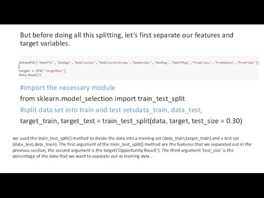
- 33. But before doing all this splitting, let’s first separate our features and target variables. #import the
- 34. Watch subtitled video https://www.coursera.org/lecture/machine-learning/what-is-machine-learning-Ujm7v
- 38. Скачать презентацию
Слайд 3.
Lecture3.
Data preproccessing and machine learning with Scikit-learn
.
Lecture3.
Data preproccessing and machine learning with Scikit-learn
Слайд 4Извлечение признаков и масшатбирование, будущая выборка, уменьшение размерности выборки
Извлечение признаков и масшатбирование, будущая выборка, уменьшение размерности выборки
Слайд 5Training set and testing set
Machine learning is about learning some properties of
Training set and testing set
Machine learning is about learning some properties of
Слайд 6Reading a Dataset
Reading a Dataset
Слайд 8Data Description :
Attribute Information:
1. sepal length in cm
2. sepal width in cm
3.
Data Description :
Attribute Information: 1. sepal length in cm 2. sepal width in cm 3.
Слайд 9A basic table is a two-dimensional grid of data, in which the
A basic table is a two-dimensional grid of data, in which the
Слайд 10Target array
In dataset we also work with a label or target array, which by convention we
Target array
In dataset we also work with a label or target array, which by convention we
Слайд 11Basic Data Analysis :
The dataset provided has 150 rows
Dependent Variables : Sepal
Basic Data Analysis :
The dataset provided has 150 rows
Dependent Variables : Sepal
Слайд 12The dataset is divided into
Train and Test data
with 80:20 split
The dataset is divided into
Train and Test data
with 80:20 split
Слайд 13Each training point belongs to one of N different classes.
The goal
Each training point belongs to one of N different classes.
The goal
Слайд 14What is scikit-learn?
The scikit-learn library provides an implementation of a range of
What is scikit-learn?
The scikit-learn library provides an implementation of a range of
Слайд 15
You can watch the Pandas and scikit-learn features documentation on this site.
https://pandas.pydata.org/pandas-docs/stable/
https://scikit-learn.org/stable/documentation.html
You can watch the Pandas and scikit-learn features documentation on this site.
https://pandas.pydata.org/pandas-docs/stable/
https://scikit-learn.org/stable/documentation.html
Слайд 16Preprocessing Data: missing data
Real world data is filled with missing values.
You
Preprocessing Data: missing data
Real world data is filled with missing values.
You
Слайд 18Method 1: Mean or Median
A common method of imputation with numeric features
Method 1: Mean or Median
A common method of imputation with numeric features
Слайд 20Imputation Method 2: Zero
Depending on where your data are coming from, a
Imputation Method 2: Zero
Depending on where your data are coming from, a
Слайд 22Imputation for Categorical Data
For categorical features, using mean, median, or zero-imputation doesn’t
Imputation for Categorical Data
For categorical features, using mean, median, or zero-imputation doesn’t

Слайд 24Imputation Method 1: Most Common Class
One approach to imputing categorical features is
Imputation Method 1: Most Common Class
One approach to imputing categorical features is
Слайд 26Imputation Method 2: “Unknown” Class
Similar to how it’s sometimes most appropriate to
Imputation Method 2: “Unknown” Class
Similar to how it’s sometimes most appropriate to
Слайд 28Column-Specific Imputation Rules
You can combine any of the above methods by imputing
Column-Specific Imputation Rules
You can combine any of the above methods by imputing
Слайд 29Preprocessing Data
If data set are strings
We saw in our initial exploration that
Preprocessing Data
If data set are strings
We saw in our initial exploration that
Слайд 30The image below represents a dataframe that has one column named ‘color’
The image below represents a dataframe that has one column named ‘color’
Слайд 31#import the necessary module
from sklearn import preprocessing
# create the Labelencoder object
le =
#import the necessary module
from sklearn import preprocessing
# create the Labelencoder object
le =
Слайд 32Training Set & Test Set
A Machine Learning algorithm needs to be trained
Training Set & Test Set
A Machine Learning algorithm needs to be trained
Слайд 33But before doing all this splitting, let’s first separate our features and
But before doing all this splitting, let’s first separate our features and
Слайд 34
Watch subtitled video
https://www.coursera.org/lecture/machine-learning/what-is-machine-learning-Ujm7v
Watch subtitled video
https://www.coursera.org/lecture/machine-learning/what-is-machine-learning-Ujm7v


 Healthcare in Russia
 Презентация на тему Этапы функции планирования
  Занятия на открытом воздухе. Организация занятий
 ФЕСТИВАЛЬ ПАТРИОТИЧЕСКОЙ ПЕСНИ
 Военные профессии в стихах и картинках
 КОМПЛЕКСНАЯ МОДЕРНИЗАЦИЯПЫЛЕУГОЛЬНЫХ КОТЛОВНА ОСНОВЕ НИЗКОТЕМПЕРАТУРНОЙ ВИХРЕВОЙ ТЕХНОЛОГИИ СЖИГАНИЯ
 Путешествие в природу
 Сочинение по картине К. Ф. Юон. «Конец зимы. Полдень»
 Kölner Dom und Ulmer Münster
 ПРЕЗЕНТАЦИЯ ПОБЕДИТЕЛЯ
 Тема: Введение. Понятие об экологии, экологии человека и медицинской экологии. Методологические проблемы, научные направления. Вз
 Ваша ультразвуковая осень
 Teorikurs 22. november
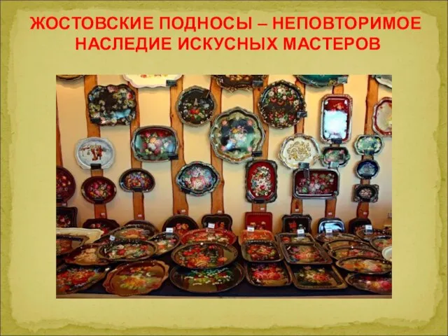 Жостовские подносы. Зачем и почему?
 Пейзажи. Рисунок морского пейзажа
 Наркотические вещества
 Река Медведица
 Органы цветкового растения
 Древние образы в народном искусстве
 Нейронные сети.
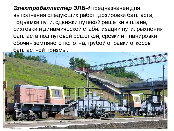 Электробалластер ЭЛБ-4
 Эстафета пионерских поколений
 Презентация на тему Ноев ковчег
 Презентация на тему Языческие верования восточных славян
  Методы управления персоналом и современные системы автоматизацииПредставление проекта
 Компьютерные обучающие программы по русскому языку
 Эмоционально-смысловой метод И.Ю. Шехтера
 Моя творческая мастерская