- Optimization models

Содержание
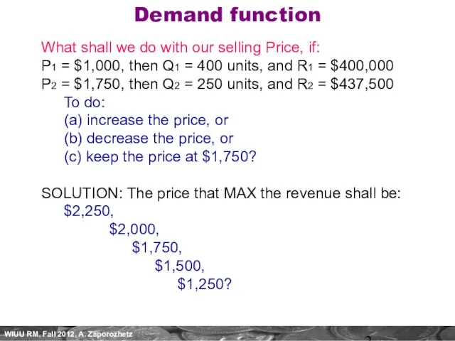
- 2. Demand function What shall we do with our selling Price, if: P1 = $1,000, then Q1
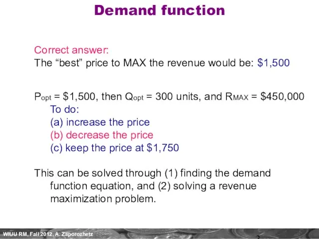
- 3. Demand function Correct answer: The “best” price to MAX the revenue would be: $1,500 Popt =
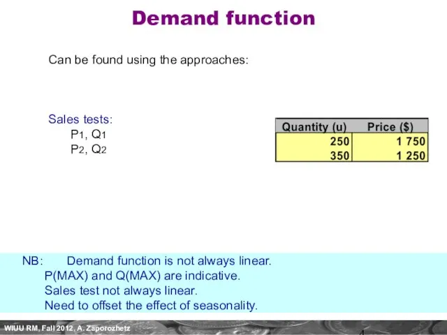
- 4. Demand function Can be found using the approaches: Sales tests: P1, Q1 P2, Q2 NB: Demand
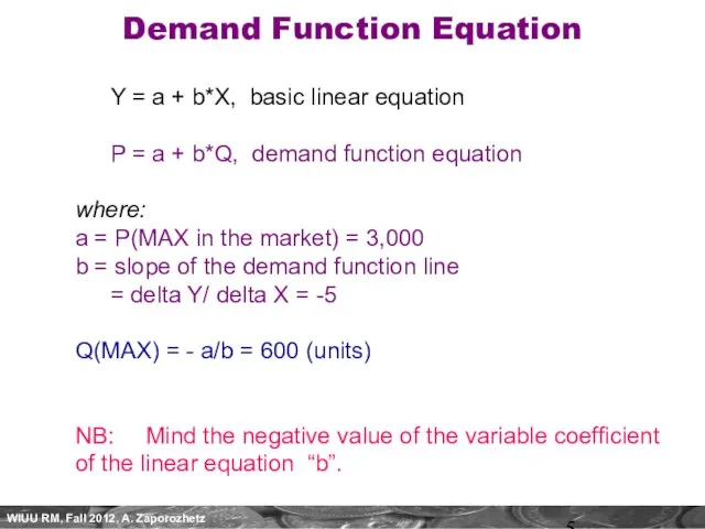
- 5. Demand Function Equation Y = a + b*X, basic linear equation P = a + b*Q,
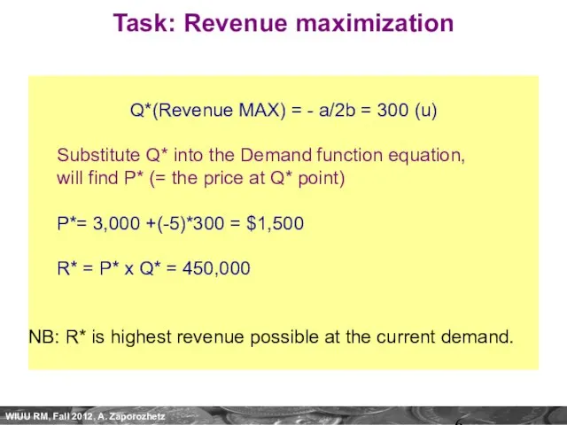
- 6. Task: Revenue maximization Q*(Revenue MAX) = - a/2b = 300 (u) Substitute Q* into the Demand
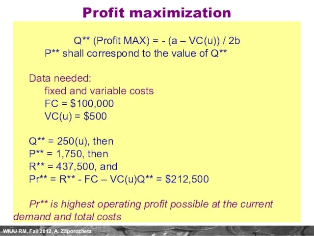
- 7. Profit maximization Q** (Profit MAX) = - (a – VC(u)) / 2b P** shall correspond to
- 9. Скачать презентацию
Слайд 3Demand function
Correct answer:
The “best” price to MAX the revenue would be:
Demand function
Correct answer:
The “best” price to MAX the revenue would be:
Слайд 4Demand function
Can be found using the approaches:
Sales tests:
P1, Q1
P2, Q2
NB: Demand
Demand function
Can be found using the approaches:
Sales tests:
P1, Q1
P2, Q2
NB: Demand
Слайд 5Demand Function Equation
Y = a + b*X, basic linear equation
P = a
Demand Function Equation
Y = a + b*X, basic linear equation
P = a
Слайд 6Task: Revenue maximization
Q*(Revenue MAX) = - a/2b = 300 (u)
Substitute Q* into
Task: Revenue maximization
Q*(Revenue MAX) = - a/2b = 300 (u)
Substitute Q* into
Слайд 7Profit maximization
Q** (Profit MAX) = - (a – VC(u)) / 2b
P** shall
Profit maximization
Q** (Profit MAX) = - (a – VC(u)) / 2b
P** shall
 ОСОБЕННОСТИ СТРОЕНИЯ, РЕАКЦИОННОЙ СПОСОБНОСТИ И МЕТОДЫ синтеза
  Управление образовательным учреждением: вводные замечания
 Информация о компании ФБК
 Кто может прийти в тренажерный зал?
 Имя существительное как часть речи
 Тайм-менеджмент для обучающихся. Приёмы эффективной организации времени
 Презентация на тему Задания с производной при подготовке к ЕГЭ Задания В8 и В14
 Архитектура. 7 чудес света
 Теория элит
 Презентация на тему методическая система
  Секреты невербальной коммуникации
 Правописание гласных в корне слова
 лаб 3
лаб 3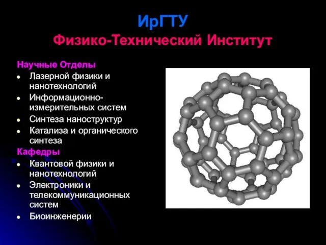 ИрГТУФизико-Технический Институт
 Введение в курс Обществознание
 Физико-географическое положение Северной Америки
 Физиология автономной нервной системы
 Российский коммерческий банк Сбербанк. Услуги банка
 Приставки при- и пре- 5 класс
 Осторожно! Сосульки!
 Типы товаров
 Пример-шаблон постера
 Дорога жизни – Ладожское озеро
 Дирижабли. Виды дирижаблей
 Презентация на тему Wir wiederhollen. Мы повторяем.
 Построение спутниковой связи на базе космических аппаратов
  Итоги работы ГОУ СОШ №237 Северо-Восточного округа в 2007-2008 учебном году
 Оценка и управление профессиональными рисками в моей организации