- Fields (functions)

Содержание
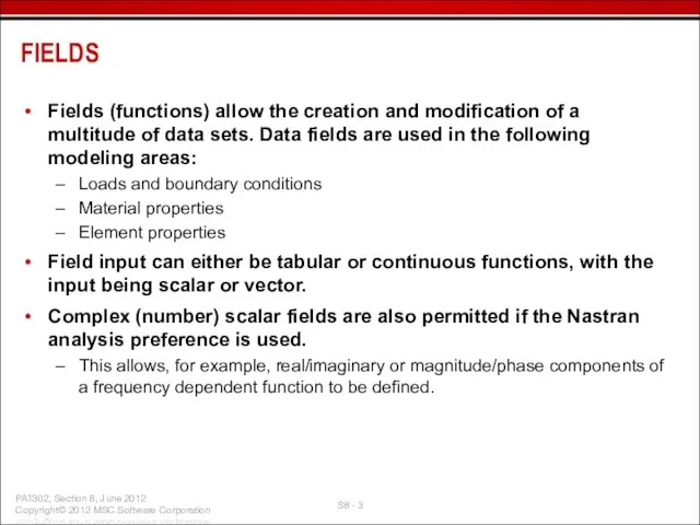
- 3. Fields (functions) allow the creation and modification of a multitude of data sets. Data fields are
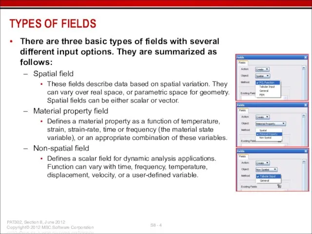
- 4. There are three basic types of fields with several different input options. They are summarized as
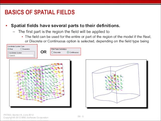
- 5. Spatial fields have several parts to their definitions. The first part is the region the field
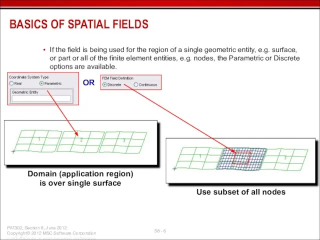
- 6. If the field is being used for the region of a single geometric entity, e.g. surface,
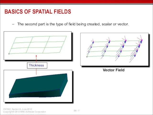
- 7. The second part is the type of field being created, scalar or vector. BASICS OF SPATIAL
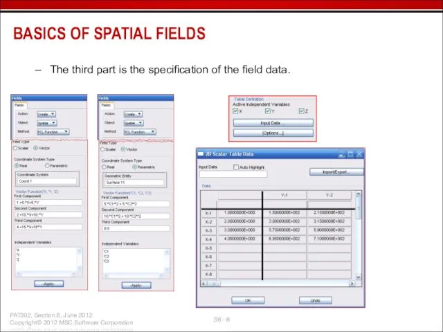
- 8. The third part is the specification of the field data. BASICS OF SPATIAL FIELDS
- 9. The third part is the specification of the field data. BASICS OF SPATIAL FIELDS Thermal Results
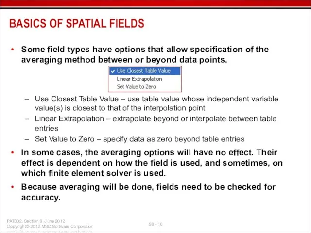
- 10. BASICS OF SPATIAL FIELDS Some field types have options that allow specification of the averaging method
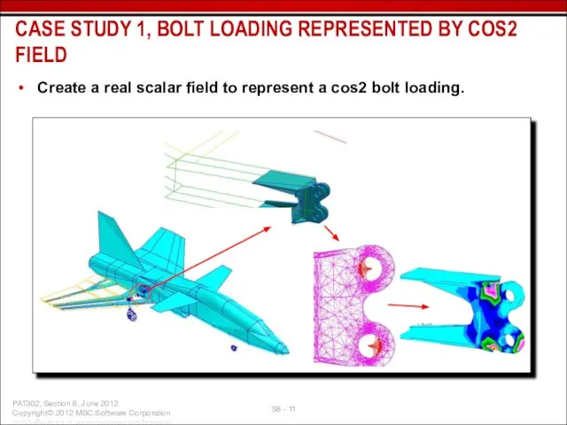
- 11. Create a real scalar field to represent a cos2 bolt loading. CASE STUDY 1, BOLT LOADING
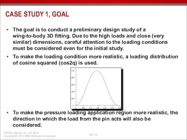
- 12. The goal is to conduct a preliminary design study of a wing-to-body 3D fitting. Due to
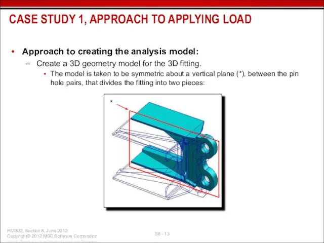
- 13. Approach to creating the analysis model: Create a 3D geometry model for the 3D fitting. The
- 14. CASE STUDY 1, APPROACH TO APPLYING LOAD Approach to creating the analysis model The applied loads
- 15. From the full aircraft model, a beam element representation of the main spares is made and
- 16. The force (both symmetric halves of the fitting are included) at the top (*) and bottom
- 17. Integrating the component of the pressure function, , in the direction of the applied load, the
- 18. Create coordinate systems at the center of the bolt holes to do the following: Specify the
- 19. Calculate the angle to rotate the coordinate frames. This will be based on the components of
- 20. Break the solid using the rotated coordinate frames. This gives the needed solid faces for applying
- 21. TetMesh the model Use mesh seeds for a finer mesh around the pin holes. Mesh the
- 22. A separate field and pressure load set needs to be created for each pin hole loading.
- 23. Scalar Function in the form has 4 key components: (cosr(‘T+3.14159/2))**2 CASE STUDY 1, CREATE THE FIELD
- 24. Verify the created field. In Fields: Show, Specify Range gives a range over which the field
- 25. If the plot or table data does not look correct, increase the number of points. Sometimes,
- 26. Create the load for the top pin. Target Element Type is 3D because solid finite elements
- 27. The application region form is set to Geometry and the solid face representing the pin contact
- 28. Display / Load/BC/Elem. Props… is used to view the pressures on the finite elements. For clarity,
- 29. The image of the finite element model (to the left) displays the pressure markers at the
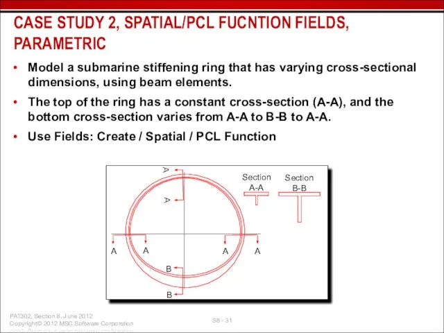
- 31. Model a submarine stiffening ring that has varying cross-sectional dimensions, using beam elements. The top of
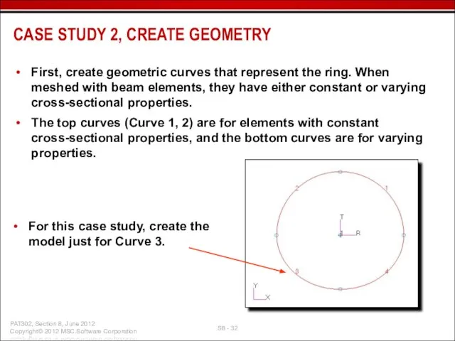
- 32. First, create geometric curves that represent the ring. When meshed with beam elements, they have either
- 33. It is necessary to create two spatially varying fields, one for the height of the cross-section,
- 34. In Properties, the dimensions of the “I” beam are specified using Beam Library. The appropriate fields
- 35. Use Display: Load/BC/Elem. Props, Beam Display to view the finished beam cross-sections in the viewport. CASE
- 36. Spatial/PCL Function, Vector is similar to Scalar except that individual direction components can be specified: Using
- 37. Use Spatial/PCL Function to make a vector field, representing a varying traction load and radial-pressure load
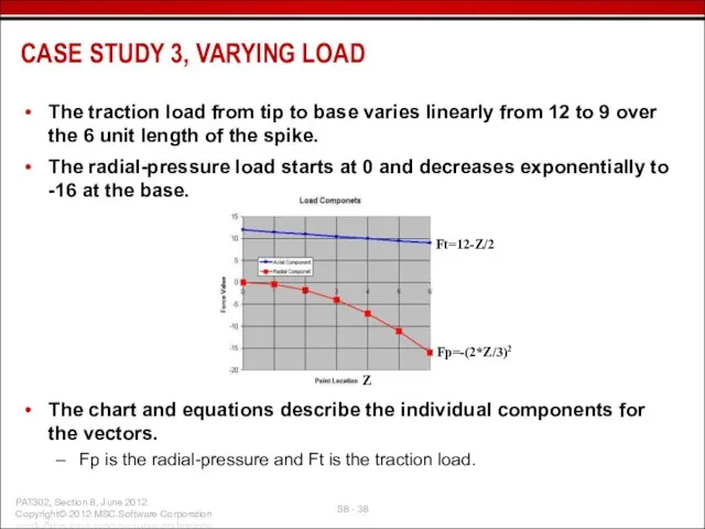
- 38. The traction load from tip to base varies linearly from 12 to 9 over the 6
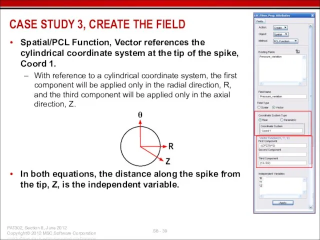
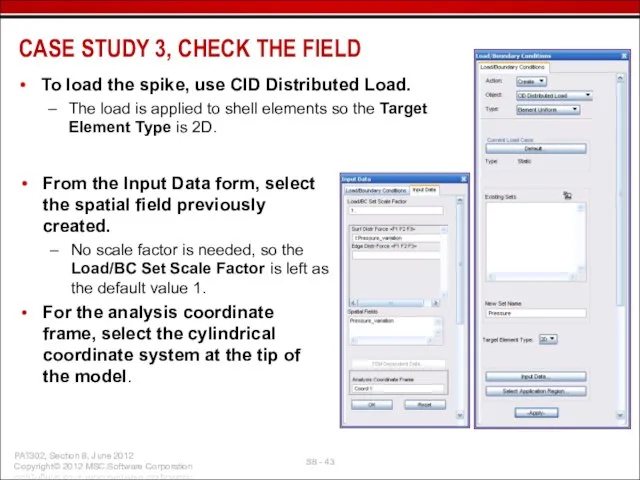
- 39. Spatial/PCL Function, Vector references the cylindrical coordinate system at the tip of the spike, Coord 1.
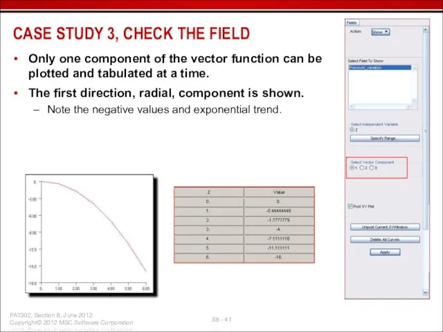
- 40. Use Fields/Show to check the equation. In the Select Independent Variable, only the Z variable is
- 41. Only one component of the vector function can be plotted and tabulated at a time. The
- 42. The third direction, axial, component is now plotted. Note the positive values and negative linear trend.
- 43. To load the spike, use CID Distributed Load. The load is applied to shell elements so
- 44. For the Select Application Region, select all the shell elements used to model the spike CASE
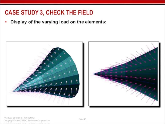
- 45. Display of the varying load on the elements: CASE STUDY 3, CHECK THE FIELD
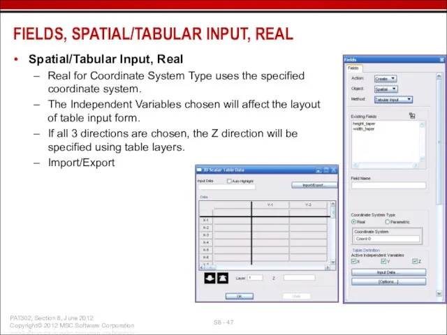
- 47. Spatial/Tabular Input, Real Real for Coordinate System Type uses the specified coordinate system. The Independent Variables
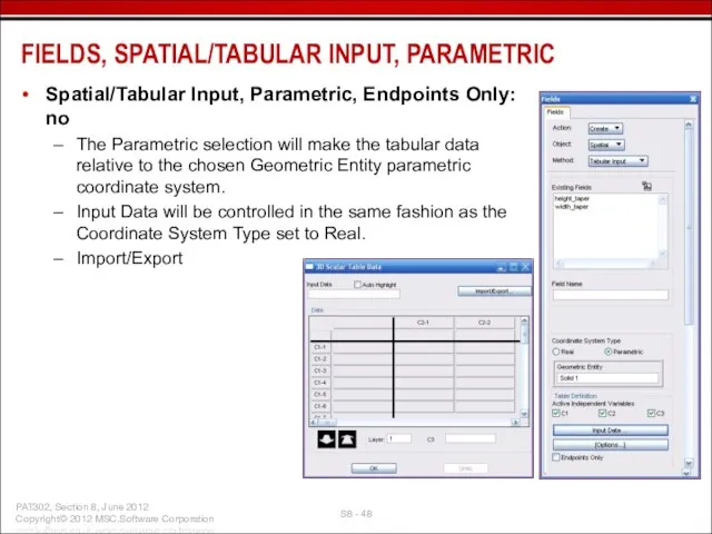
- 48. Spatial/Tabular Input, Parametric, Endpoints Only: no The Parametric selection will make the tabular data relative to
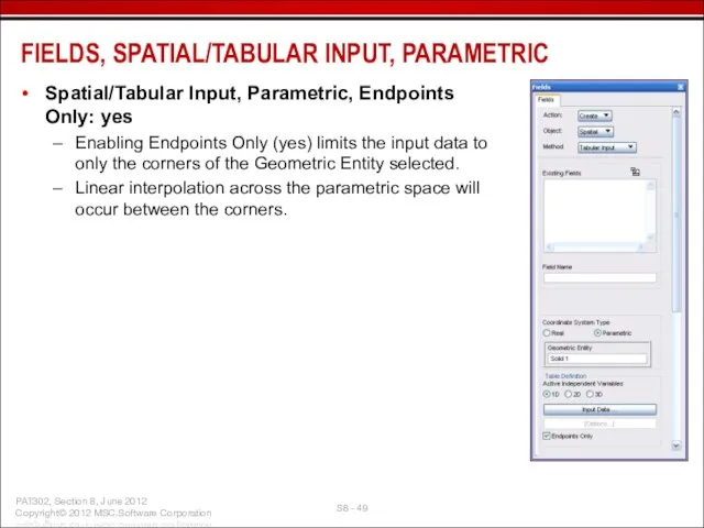
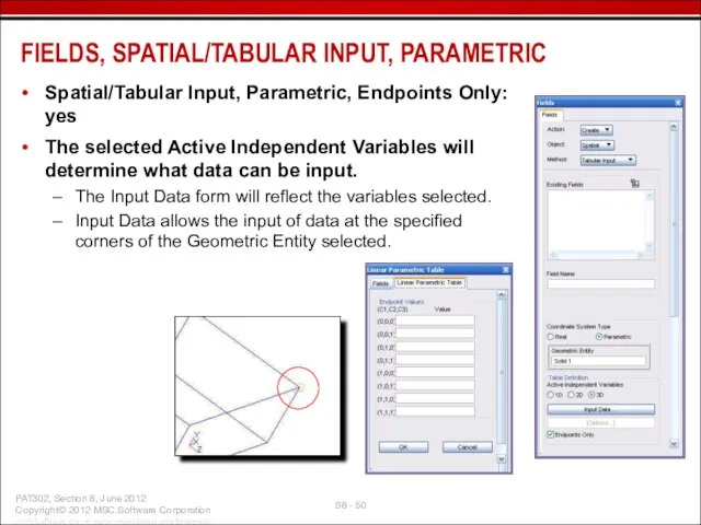
- 49. Spatial/Tabular Input, Parametric, Endpoints Only: yes Enabling Endpoints Only (yes) limits the input data to only
- 50. Spatial/Tabular Input, Parametric, Endpoints Only: yes The selected Active Independent Variables will determine what data can
- 51. Spatial/Tabular Input, [Options] The top portion of the Tabular Input, [Options] controls how many data points
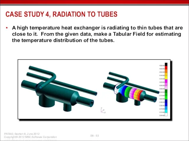
- 53. A high temperature heat exchanger is radiating to thin tubes that are close to it. From
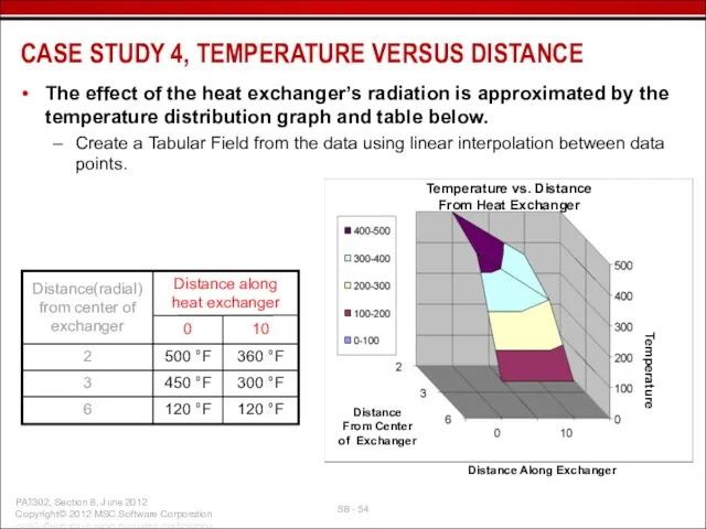
- 54. The effect of the heat exchanger’s radiation is approximated by the temperature distribution graph and table
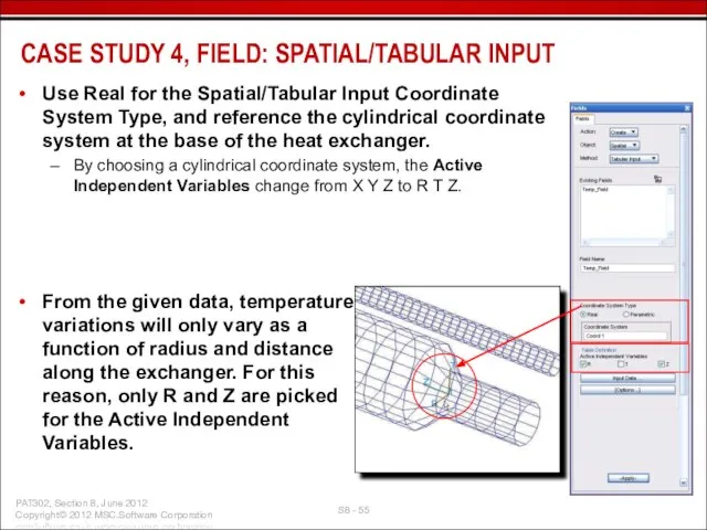
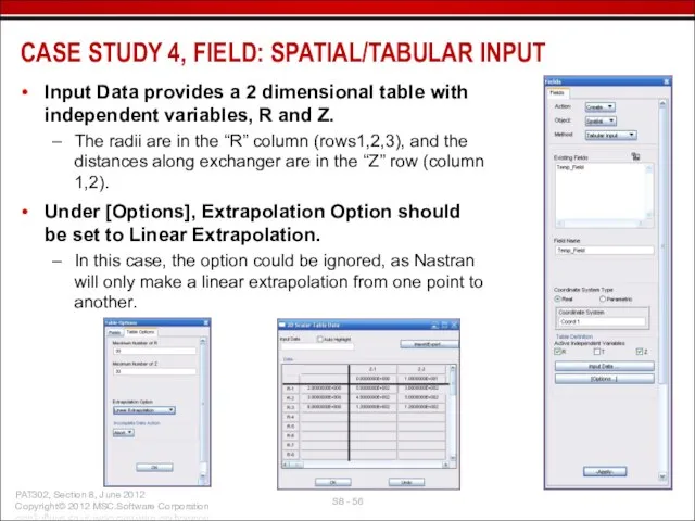
- 55. CASE STUDY 4, FIELD: SPATIAL/TABULAR INPUT Use Real for the Spatial/Tabular Input Coordinate System Type, and
- 56. Input Data provides a 2 dimensional table with independent variables, R and Z. The radii are
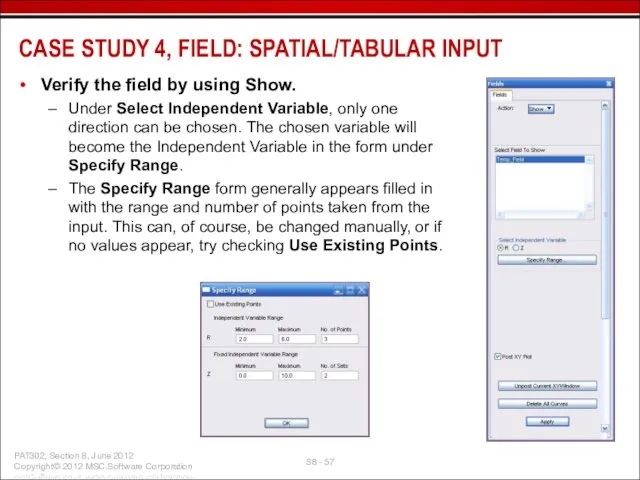
- 57. Verify the field by using Show. Under Select Independent Variable, only one direction can be chosen.
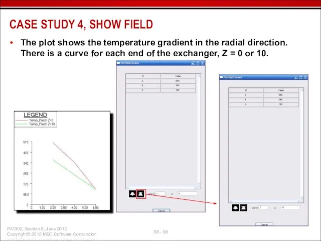
- 58. The plot shows the temperature gradient in the radial direction. There is a curve for each
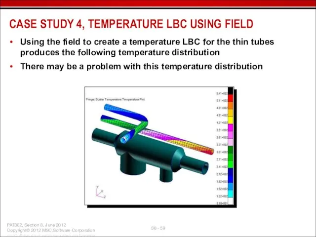
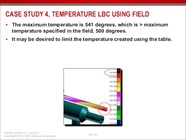
- 59. Using the field to create a temperature LBC for the thin tubes produces the following temperature
- 60. The maximum temperature is 541 degrees, which is > maximum temperature specified in the field, 500
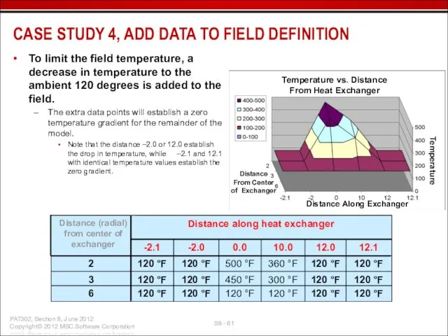
- 61. Distance From Center of Exchanger 120 °F 300 °F 360 °F 10.0 120 °F 120 °F
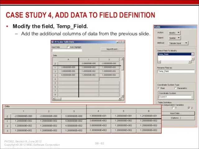
- 62. Modify the field, Temp_Field. Add the additional columns of data from the previous slide. CASE STUDY
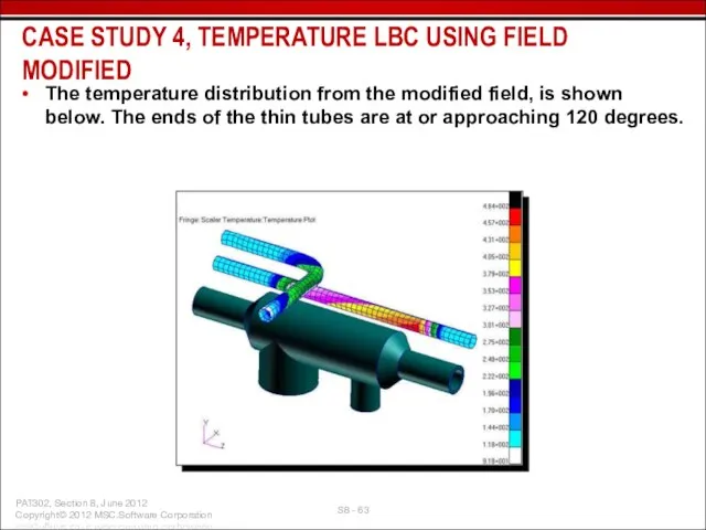
- 63. The temperature distribution from the modified field, is shown below. The ends of the thin tubes
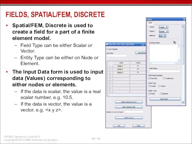
- 65. Spatial/FEM, Discrete is used to create a field for a part of a finite element model.
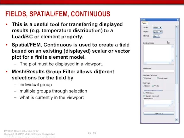
- 66. This is a useful tool for transferring displayed results (e.g. temperature distribution) to a Load/BC or
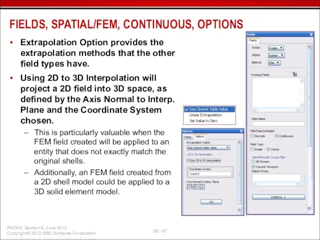
- 67. Extrapolation Option provides the extrapolation methods that the other field types have. Using 2D to 3D
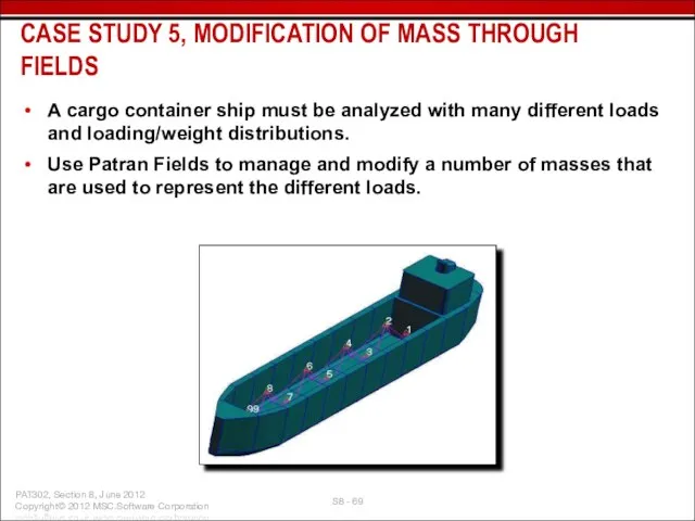
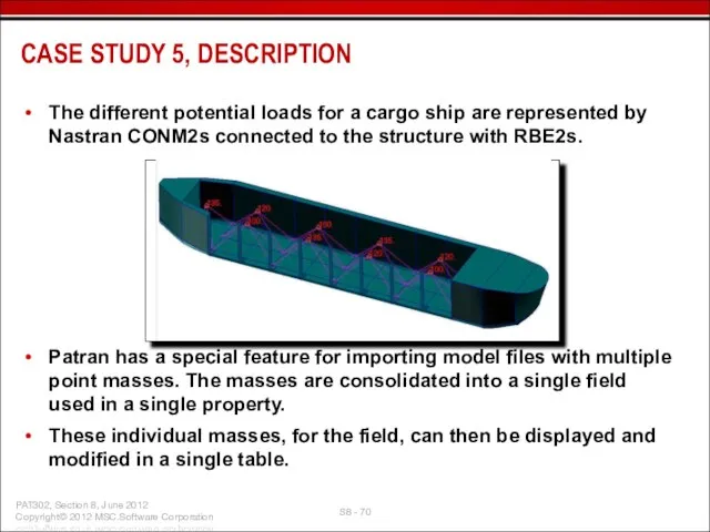
- 69. A cargo container ship must be analyzed with many different loads and loading/weight distributions. Use Patran
- 70. The different potential loads for a cargo ship are represented by Nastran CONM2s connected to the
- 71. In this case study, the point masses are first created in Patran Properties: Create / 0D
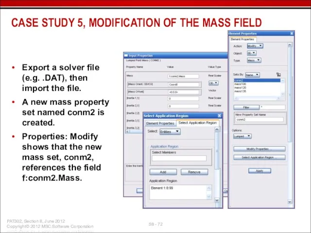
- 72. Export a solver file (e.g. .DAT), then import the file. A new mass property set named
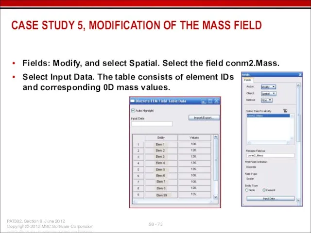
- 73. Fields: Modify, and select Spatial. Select the field conm2.Mass. Select Input Data. The table consists of
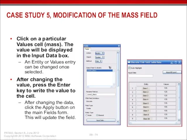
- 74. Click on a particular Values cell (mass). The value will be displayed in the Input Data
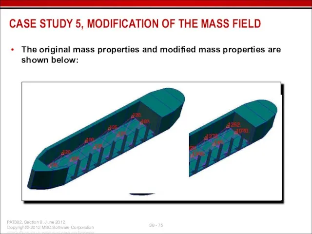
- 75. The original mass properties and modified mass properties are shown below: CASE STUDY 5, MODIFICATION OF
- 76. For this case study, individual properties (e.g. mass135, mass=135, Point 266, 291, 293) were first created,
- 77. CASE STUDY 6 FEM FIELD, CONTINUOUS CFD PRESSURE TO PATRAN PRESSURE
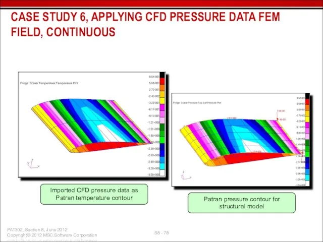
- 78. CASE STUDY 6, APPLYING CFD PRESSURE DATA FEM FIELD, CONTINUOUS Imported CFD pressure data as Patran
- 79. This case study demonstrates the use of FEM Field, Continuous as a way of creating an
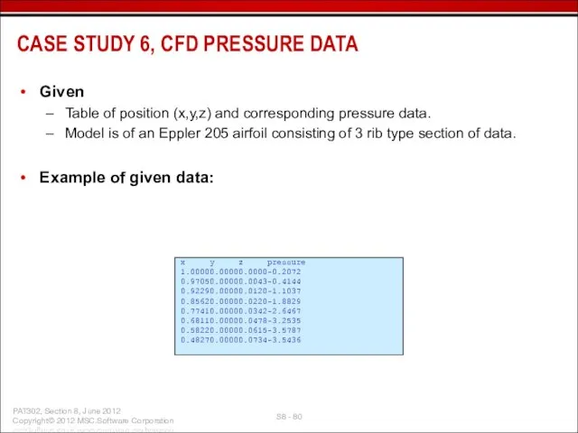
- 80. Given Table of position (x,y,z) and corresponding pressure data. Model is of an Eppler 205 airfoil
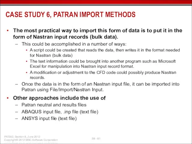
- 81. The most practical way to import this form of data is to put it in the
- 82. In this example, Microsoft Excel is used. Below, is a screen snap-shot of the raw data
- 83. Second sheet Location (x,y,z) data Third sheet Pressure data CASE STUDY 6, CREATE NASTRAN INPUT FILE
- 84. Once the data is arranged, write it to a text file(s). Once the text file(s) is
- 85. Imported Nastran grid points, called Patran nodes. CASE STUDY 6, VERIFY IMPORTED NASTRAN INPUT FILE DATA
- 86. Under Loads/BCs, the temperature should be plotted to make sure the data is correct. If Tempe_temp.1
- 87. Use the temperature information in Patran to create pressure for a structural model. This is done
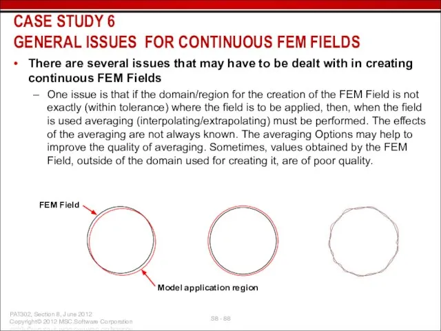
- 88. There are several issues that may have to be dealt with in creating continuous FEM Fields
- 89. (Continued) This issue can be partially resolved for 2D models by enabling an Option to extend
- 90. Another issue with creating FEM Fields is that this type of field must be created from
- 91. Attempts have been made to make an FEM Field with 1D elements that connected all the
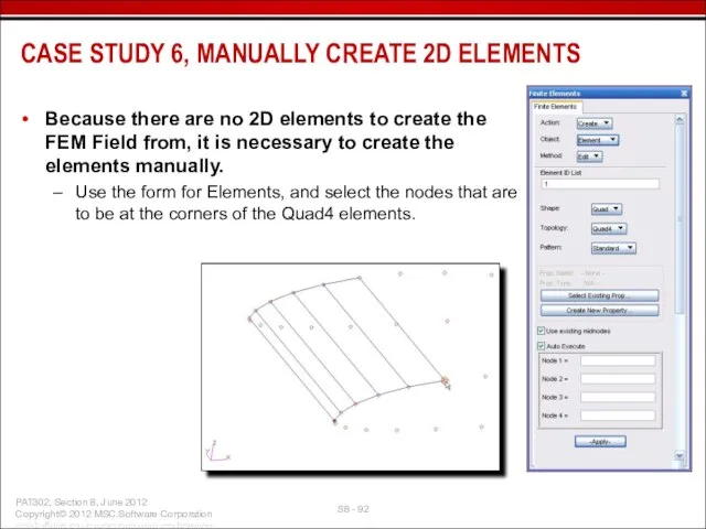
- 92. Because there are no 2D elements to create the FEM Field from, it is necessary to
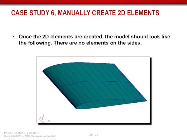
- 93. Once the 2D elements are created, the model should look like the following. There are no
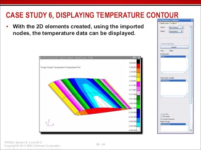
- 94. With the 2D elements created, using the imported nodes, the temperature data can be displayed. CASE
- 95. Create the FEM Field using the posted temperature fringe. Fill out the Fields menu as shown,
- 96. Looking ahead, the consequences of ignoring the surface overlap can be seen. Notice that the pressure
- 97. To make the FEM Field correctly, simply put the top and bottom surfaces (of elements) in
- 98. Create the pressure LBCs using the two FEM Fields. Loads/BCs: Create/Pressure/Element Uniform Input Data Select one
- 99. Perform Workshop 19 “Global/Local Modeling Using FEM Fields” in your exercise workbook. EXERCISES
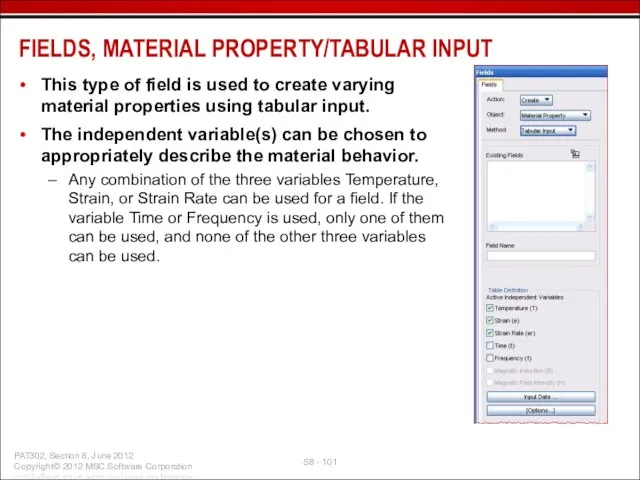
- 101. This type of field is used to create varying material properties using tabular input. The independent
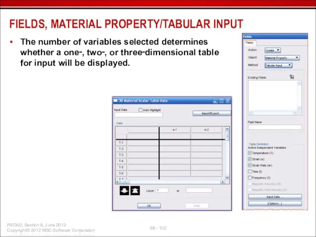
- 102. The number of variables selected determines whether a one‑, two‑, or three‑dimensional table for input will
- 103. The top portion of the Tabular Input, [Options] form controls how many data points can be
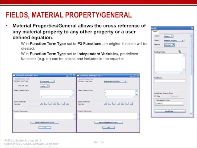
- 104. Material Properties/General allows the cross reference of any material property to any other property or a
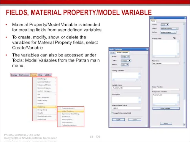
- 105. Material Property/Model Variable is intended for creating fields from user defined variables. To create, modify, show,
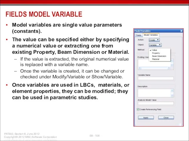
- 106. Model variables are single value parameters (constants). The value can be specified either by specifying a
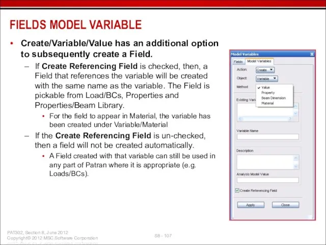
- 107. Create/Variable/Value has an additional option to subsequently create a Field. If Create Referencing Field is checked,
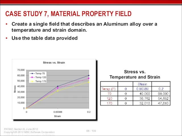
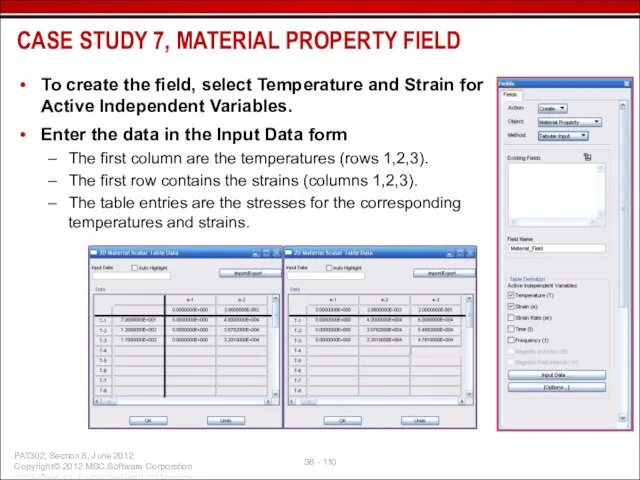
- 109. Stress vs. Temperature and Strain Create a single field that describes an Aluminum alloy over a
- 110. CASE STUDY 7, MATERIAL PROPERTY FIELD To create the field, select Temperature and Strain for Active
- 111. In [Options] the Extrapolation Option chosen does not affect the field evaluation for the Nastran preference.
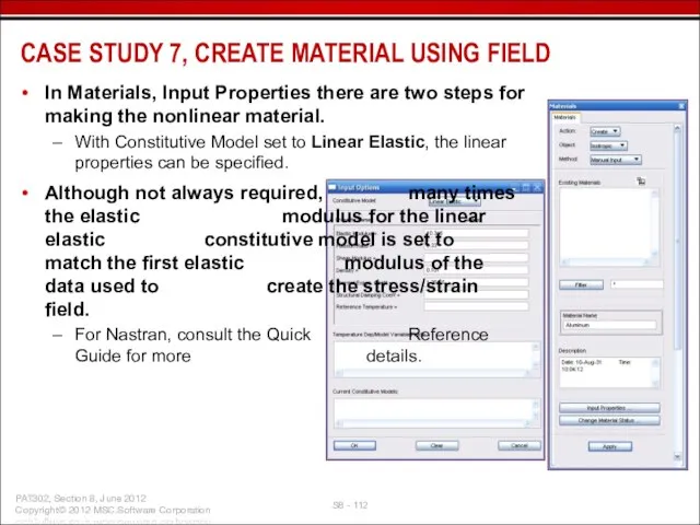
- 112. In Materials, Input Properties there are two steps for making the nonlinear material. With Constitutive Model
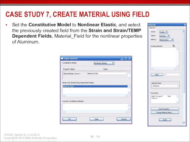
- 113. Set the Constitutive Model to Nonlinear Elastic, and select the previously created field from the Strain
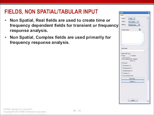
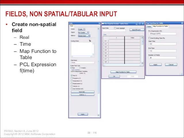
- 115. Non Spatial, Real fields are used to create time or frequency dependent fields for transient or
- 116. Create non-spatial field Real Time Map Function to Table PCL Expression f(time) FIELDS, NON SPATIAL/TABULAR INPUT
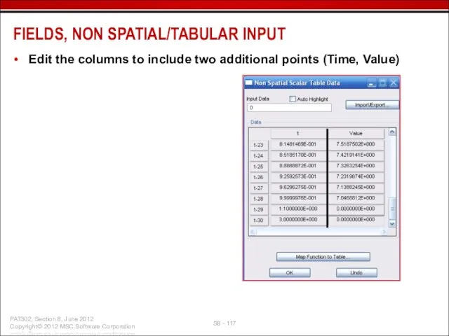
- 117. Edit the columns to include two additional points (Time, Value) FIELDS, NON SPATIAL/TABULAR INPUT
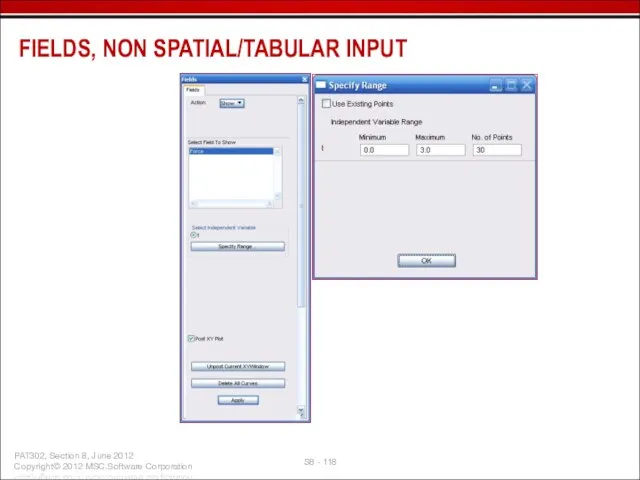
- 118. FIELDS, NON SPATIAL/TABULAR INPUT
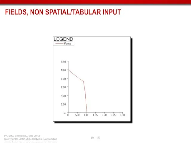
- 119. FIELDS, NON SPATIAL/TABULAR INPUT
- 121. Скачать презентацию

Слайд 3Fields (functions) allow the creation and modification of a multitude of data
Fields (functions) allow the creation and modification of a multitude of data
Слайд 4There are three basic types of fields with several different input options.
There are three basic types of fields with several different input options.
Слайд 5Spatial fields have several parts to their definitions.
The first part is
Spatial fields have several parts to their definitions.
The first part is
Слайд 6If the field is being used for the region of a single
If the field is being used for the region of a single
Слайд 7The second part is the type of field being created, scalar or
The second part is the type of field being created, scalar or
Слайд 8The third part is the specification of the field data.
BASICS OF SPATIAL
The third part is the specification of the field data.
BASICS OF SPATIAL
Слайд 9The third part is the specification of the field data.
BASICS OF SPATIAL
The third part is the specification of the field data.
BASICS OF SPATIAL

Слайд 10BASICS OF SPATIAL FIELDS
Some field types have options that allow specification of
BASICS OF SPATIAL FIELDS
Some field types have options that allow specification of
Слайд 11Create a real scalar field to represent a cos2 bolt loading.
CASE STUDY
Create a real scalar field to represent a cos2 bolt loading.
CASE STUDY
Слайд 12The goal is to conduct a preliminary design study of a wing-to-body
The goal is to conduct a preliminary design study of a wing-to-body
Слайд 13Approach to creating the analysis model:
Create a 3D geometry model for the
Approach to creating the analysis model:
Create a 3D geometry model for the
Слайд 14CASE STUDY 1, APPROACH TO APPLYING LOAD
Approach to creating the analysis model
The
CASE STUDY 1, APPROACH TO APPLYING LOAD
Approach to creating the analysis model
The
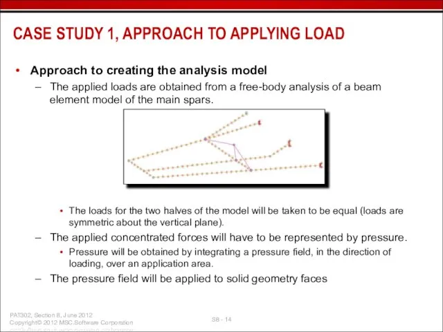
Слайд 15From the full aircraft model, a beam element representation of the main
From the full aircraft model, a beam element representation of the main
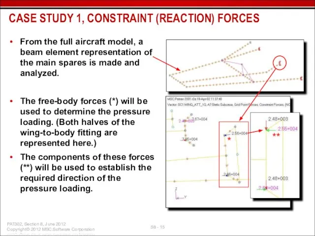
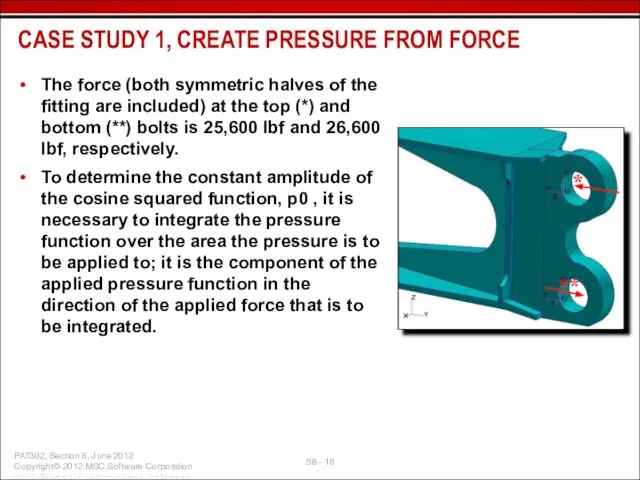
Слайд 16The force (both symmetric halves of the fitting are included) at the
The force (both symmetric halves of the fitting are included) at the
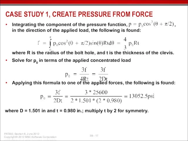
Слайд 17Integrating the component of the pressure function, , in the direction of
Integrating the component of the pressure function, , in the direction of
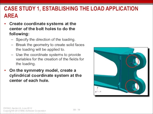
Слайд 18Create coordinate systems at the center of the bolt holes to do
Create coordinate systems at the center of the bolt holes to do
Слайд 19Calculate the angle to rotate the coordinate frames. This will be based
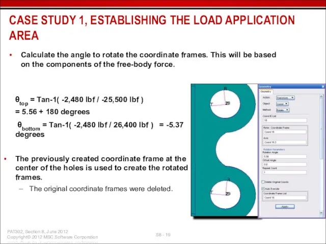
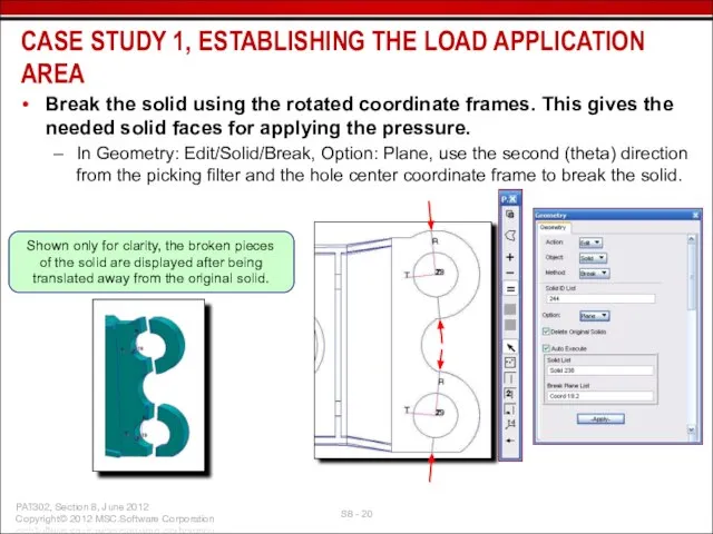
Слайд 20Break the solid using the rotated coordinate frames. This gives the needed
Break the solid using the rotated coordinate frames. This gives the needed
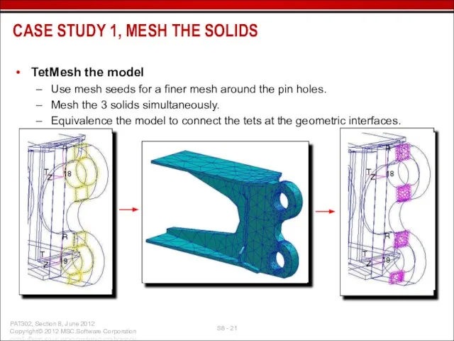
Слайд 21TetMesh the model
Use mesh seeds for a finer mesh around the pin
TetMesh the model
Use mesh seeds for a finer mesh around the pin
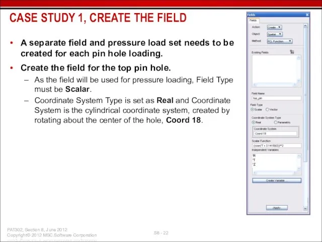
Слайд 22A separate field and pressure load set needs to be created for
A separate field and pressure load set needs to be created for
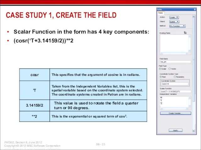
Слайд 23Scalar Function in the form has 4 key components:
(cosr(‘T+3.14159/2))**2
CASE STUDY 1, CREATE
Scalar Function in the form has 4 key components:
(cosr(‘T+3.14159/2))**2
CASE STUDY 1, CREATE
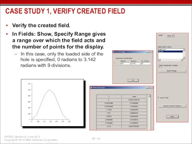
Слайд 24Verify the created field.
In Fields: Show, Specify Range gives a range over
Verify the created field.
In Fields: Show, Specify Range gives a range over
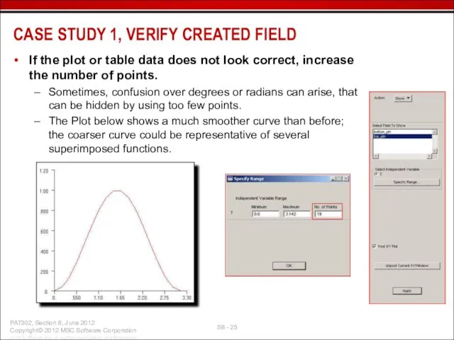
Слайд 25If the plot or table data does not look correct, increase the
If the plot or table data does not look correct, increase the
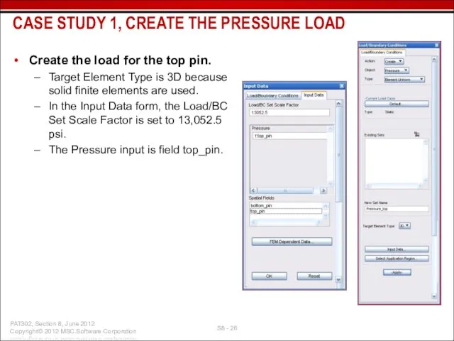
Слайд 26Create the load for the top pin.
Target Element Type is 3D because
Create the load for the top pin.
Target Element Type is 3D because
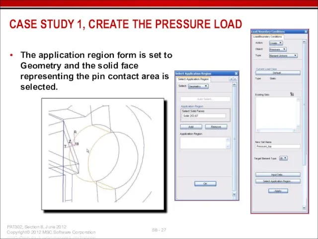
Слайд 27The application region form is set to Geometry and the solid face
The application region form is set to Geometry and the solid face
Слайд 28Display / Load/BC/Elem. Props… is used to view the pressures on the
Display / Load/BC/Elem. Props… is used to view the pressures on the
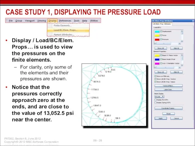
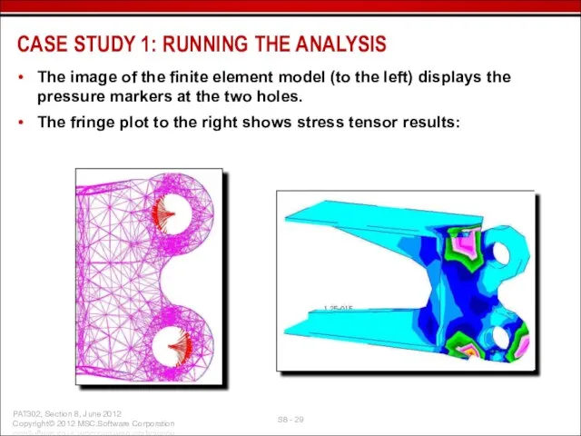
Слайд 29The image of the finite element model (to the left) displays the
The image of the finite element model (to the left) displays the

Слайд 31Model a submarine stiffening ring that has varying cross-sectional dimensions, using beam
Model a submarine stiffening ring that has varying cross-sectional dimensions, using beam
Слайд 32First, create geometric curves that represent the ring. When meshed with beam
First, create geometric curves that represent the ring. When meshed with beam
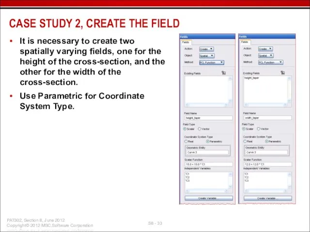
Слайд 33It is necessary to create two spatially varying fields, one for the
It is necessary to create two spatially varying fields, one for the
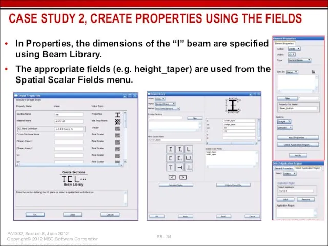
Слайд 34In Properties, the dimensions of the “I” beam are specified using Beam
In Properties, the dimensions of the “I” beam are specified using Beam
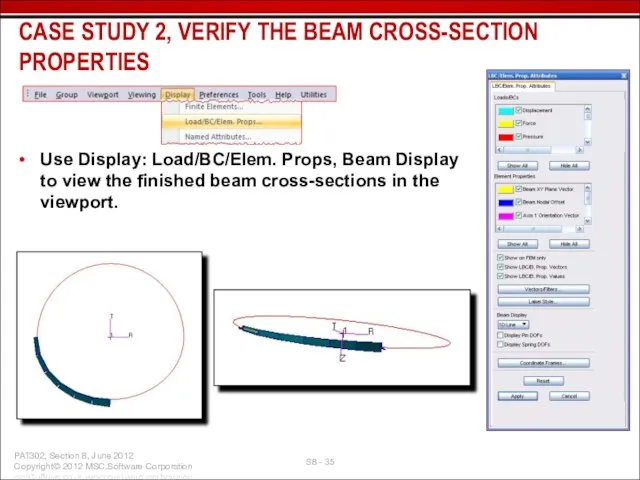
Слайд 35Use Display: Load/BC/Elem. Props, Beam Display to view the finished beam cross-sections
Use Display: Load/BC/Elem. Props, Beam Display to view the finished beam cross-sections
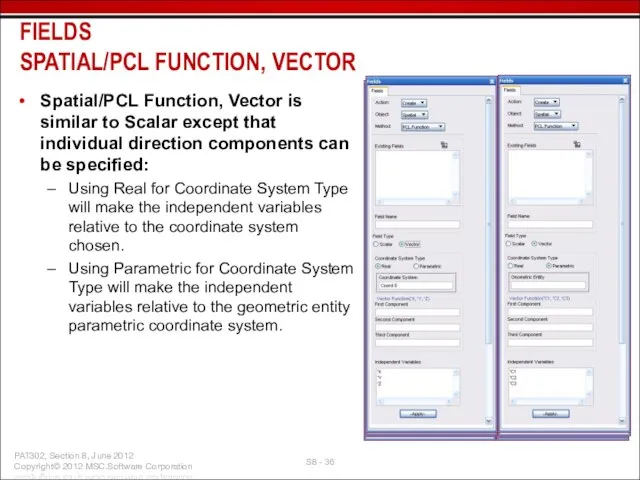
Слайд 36Spatial/PCL Function, Vector is similar to Scalar except that individual direction components
Spatial/PCL Function, Vector is similar to Scalar except that individual direction components
Слайд 37Use Spatial/PCL Function to make a vector field, representing a varying traction
Use Spatial/PCL Function to make a vector field, representing a varying traction
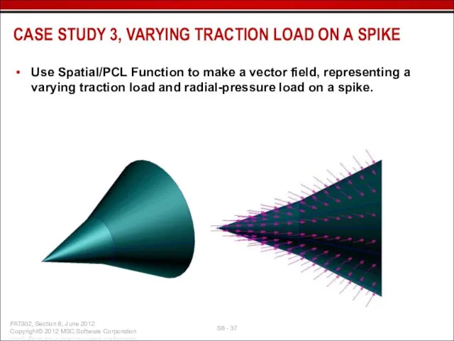
Слайд 38The traction load from tip to base varies linearly from 12 to
The traction load from tip to base varies linearly from 12 to
Слайд 39Spatial/PCL Function, Vector references the cylindrical coordinate system at the tip of
Spatial/PCL Function, Vector references the cylindrical coordinate system at the tip of
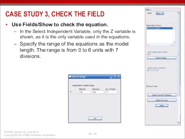
Слайд 40Use Fields/Show to check the equation.
In the Select Independent Variable, only the
Use Fields/Show to check the equation.
In the Select Independent Variable, only the
Слайд 41Only one component of the vector function can be plotted and tabulated
Only one component of the vector function can be plotted and tabulated
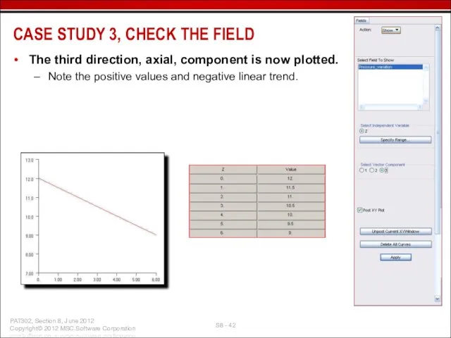
Слайд 42The third direction, axial, component is now plotted.
Note the positive values and
The third direction, axial, component is now plotted.
Note the positive values and
Слайд 43To load the spike, use CID Distributed Load.
The load is applied to
To load the spike, use CID Distributed Load.
The load is applied to
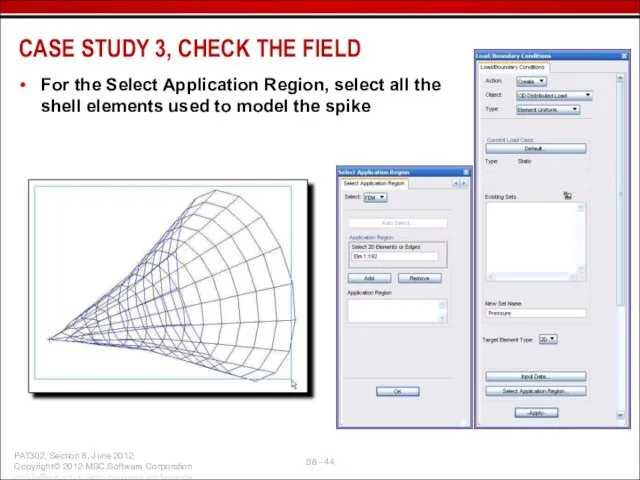
Слайд 44For the Select Application Region, select all the shell elements used to
For the Select Application Region, select all the shell elements used to
Слайд 45Display of the varying load on the elements:
CASE STUDY 3, CHECK THE
Display of the varying load on the elements:
CASE STUDY 3, CHECK THE

Слайд 47Spatial/Tabular Input, Real
Real for Coordinate System Type uses the specified coordinate
Spatial/Tabular Input, Real
Real for Coordinate System Type uses the specified coordinate
Слайд 48Spatial/Tabular Input, Parametric, Endpoints Only: no
The Parametric selection will make the tabular
Spatial/Tabular Input, Parametric, Endpoints Only: no
The Parametric selection will make the tabular
Слайд 49Spatial/Tabular Input, Parametric, Endpoints Only: yes
Enabling Endpoints Only (yes) limits the input
Spatial/Tabular Input, Parametric, Endpoints Only: yes
Enabling Endpoints Only (yes) limits the input
Слайд 50Spatial/Tabular Input, Parametric, Endpoints Only: yes
The selected Active Independent Variables will
Spatial/Tabular Input, Parametric, Endpoints Only: yes
The selected Active Independent Variables will
Слайд 51Spatial/Tabular Input, [Options]
The top portion of the Tabular Input, [Options] controls how
Spatial/Tabular Input, [Options]
The top portion of the Tabular Input, [Options] controls how
![Spatial/Tabular Input, [Options] The top portion of the Tabular Input, [Options] controls](/_ipx/f_webp&q_80&fit_contain&s_1440x1080/imagesDir/jpg/378814/slide-50.jpg)

Слайд 53A high temperature heat exchanger is radiating to thin tubes that are
A high temperature heat exchanger is radiating to thin tubes that are
Слайд 54The effect of the heat exchanger’s radiation is approximated by the temperature
The effect of the heat exchanger’s radiation is approximated by the temperature
Слайд 55CASE STUDY 4, FIELD: SPATIAL/TABULAR INPUT
Use Real for the Spatial/Tabular Input Coordinate
CASE STUDY 4, FIELD: SPATIAL/TABULAR INPUT
Use Real for the Spatial/Tabular Input Coordinate
Слайд 56Input Data provides a 2 dimensional table with independent variables, R and
Input Data provides a 2 dimensional table with independent variables, R and
Слайд 57Verify the field by using Show.
Under Select Independent Variable, only one direction
Verify the field by using Show.
Under Select Independent Variable, only one direction
Слайд 58The plot shows the temperature gradient in the radial direction. There is
The plot shows the temperature gradient in the radial direction. There is
Слайд 59Using the field to create a temperature LBC for the thin tubes
Using the field to create a temperature LBC for the thin tubes
Слайд 60The maximum temperature is 541 degrees, which is > maximum temperature specified
The maximum temperature is 541 degrees, which is > maximum temperature specified
Слайд 61Distance From Center of Exchanger
120 °F
300 °F
360 °F
10.0
120 °F
120 °F
120 °F
12.0
120 °F
450
Distance From Center of Exchanger
120 °F
300 °F
360 °F
10.0
120 °F
120 °F
120 °F
12.0
120 °F
450
Слайд 62Modify the field, Temp_Field.
Add the additional columns of data from the previous
Modify the field, Temp_Field.
Add the additional columns of data from the previous
Слайд 63The temperature distribution from the modified field, is shown below. The ends
The temperature distribution from the modified field, is shown below. The ends

Слайд 65Spatial/FEM, Discrete is used to create a field for a part of
Spatial/FEM, Discrete is used to create a field for a part of
Слайд 66This is a useful tool for transferring displayed results (e.g. temperature distribution)
This is a useful tool for transferring displayed results (e.g. temperature distribution)
Слайд 67Extrapolation Option provides the extrapolation methods that the other field types have.
Using
Extrapolation Option provides the extrapolation methods that the other field types have.
Using

Слайд 69A cargo container ship must be analyzed with many different loads and
A cargo container ship must be analyzed with many different loads and
Слайд 70The different potential loads for a cargo ship are represented by Nastran
The different potential loads for a cargo ship are represented by Nastran
Слайд 71In this case study, the point masses are first created in Patran
In this case study, the point masses are first created in Patran

Слайд 72Export a solver file (e.g. .DAT), then import the file.
A new mass
Export a solver file (e.g. .DAT), then import the file.
A new mass
Слайд 73Fields: Modify, and select Spatial. Select the field conm2.Mass.
Select Input Data.
Fields: Modify, and select Spatial. Select the field conm2.Mass.
Select Input Data.
Слайд 74Click on a particular Values cell (mass). The value will be displayed
Click on a particular Values cell (mass). The value will be displayed
Слайд 75The original mass properties and modified mass properties are shown below:
CASE STUDY
The original mass properties and modified mass properties are shown below:
CASE STUDY
Слайд 76For this case study, individual properties (e.g. mass135, mass=135, Point 266, 291,
For this case study, individual properties (e.g. mass135, mass=135, Point 266, 291,
Слайд 77CASE STUDY 6
FEM FIELD, CONTINUOUS
CFD PRESSURE TO PATRAN PRESSURE
CASE STUDY 6
FEM FIELD, CONTINUOUS
CFD PRESSURE TO PATRAN PRESSURE
Слайд 78CASE STUDY 6, APPLYING CFD PRESSURE DATA FEM FIELD, CONTINUOUS
Imported CFD pressure
CASE STUDY 6, APPLYING CFD PRESSURE DATA FEM FIELD, CONTINUOUS
Imported CFD pressure
Слайд 79This case study demonstrates the use of FEM Field, Continuous as a
This case study demonstrates the use of FEM Field, Continuous as a
Слайд 80Given
Table of position (x,y,z) and corresponding pressure data.
Model is of an Eppler
Given
Table of position (x,y,z) and corresponding pressure data.
Model is of an Eppler
Слайд 81The most practical way to import this form of data is to
The most practical way to import this form of data is to
Слайд 82In this example, Microsoft Excel is used. Below, is a screen snap-shot
In this example, Microsoft Excel is used. Below, is a screen snap-shot
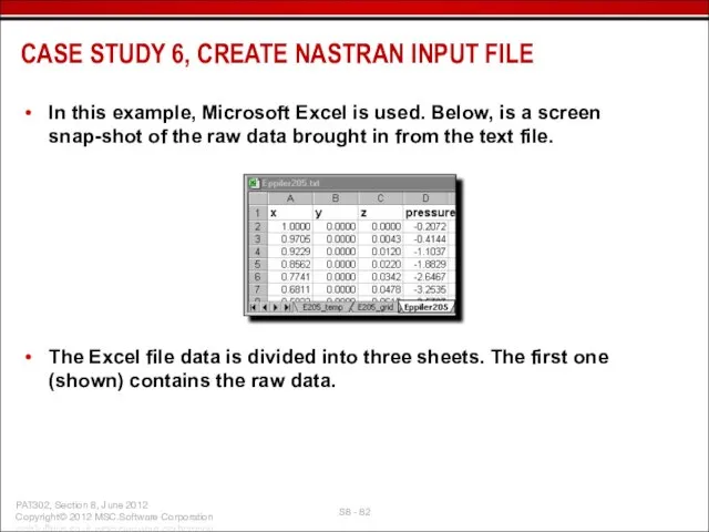
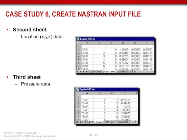
Слайд 83Second sheet
Location (x,y,z) data
Third sheet
Pressure data
CASE STUDY 6, CREATE NASTRAN INPUT FILE
Second sheet
Location (x,y,z) data
Third sheet
Pressure data
CASE STUDY 6, CREATE NASTRAN INPUT FILE
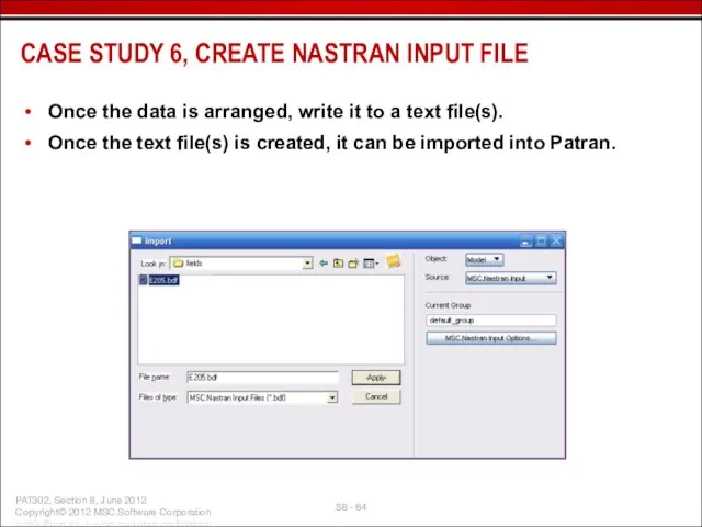
Слайд 84Once the data is arranged, write it to a text file(s).
Once the
Once the data is arranged, write it to a text file(s).
Once the
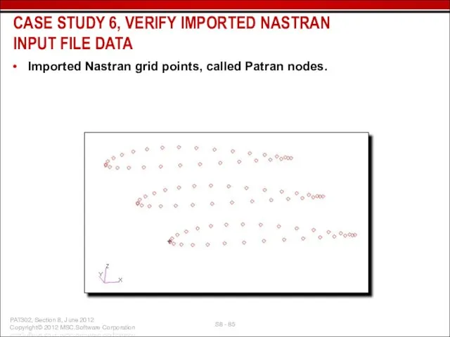
Слайд 85Imported Nastran grid points, called Patran nodes.
CASE STUDY 6, VERIFY IMPORTED NASTRAN
Imported Nastran grid points, called Patran nodes.
CASE STUDY 6, VERIFY IMPORTED NASTRAN
Слайд 86Under Loads/BCs, the temperature should be plotted to make sure the data
Under Loads/BCs, the temperature should be plotted to make sure the data
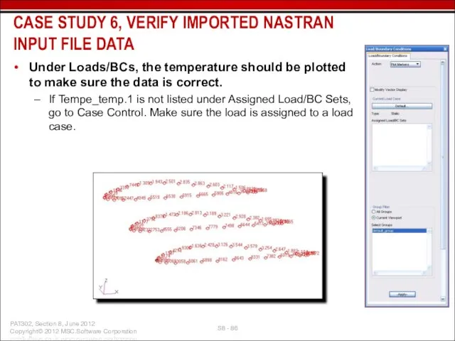
Слайд 87Use the temperature information in Patran to create pressure for a structural
Use the temperature information in Patran to create pressure for a structural
Слайд 88There are several issues that may have to be dealt with in
There are several issues that may have to be dealt with in
Слайд 89(Continued) This issue can be partially resolved for 2D models by enabling
(Continued) This issue can be partially resolved for 2D models by enabling
Слайд 90Another issue with creating FEM Fields is that this type of field
Another issue with creating FEM Fields is that this type of field
Слайд 91Attempts have been made to make an FEM Field with 1D elements
Attempts have been made to make an FEM Field with 1D elements
Слайд 92Because there are no 2D elements to create the FEM Field from,
Because there are no 2D elements to create the FEM Field from,
Слайд 93Once the 2D elements are created, the model should look like the
Once the 2D elements are created, the model should look like the
Слайд 94With the 2D elements created, using the imported nodes, the temperature data
With the 2D elements created, using the imported nodes, the temperature data
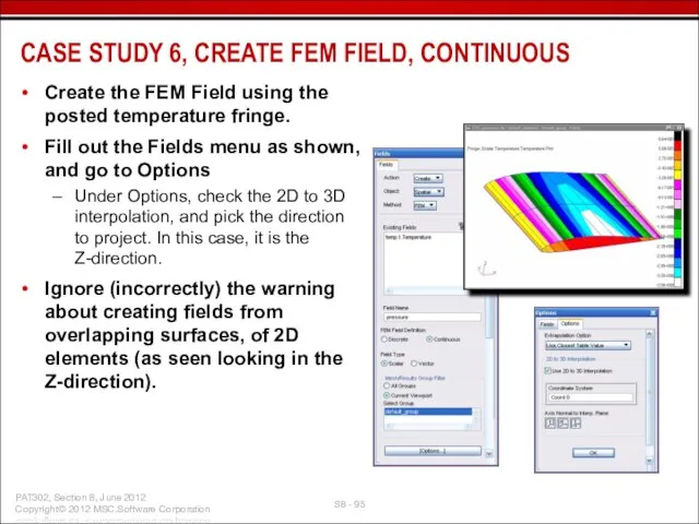
Слайд 95Create the FEM Field using the posted temperature fringe.
Fill out the
Create the FEM Field using the posted temperature fringe.
Fill out the
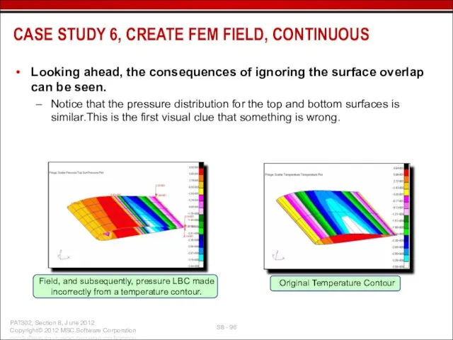
Слайд 96Looking ahead, the consequences of ignoring the surface overlap can be seen.
Notice
Looking ahead, the consequences of ignoring the surface overlap can be seen.
Notice
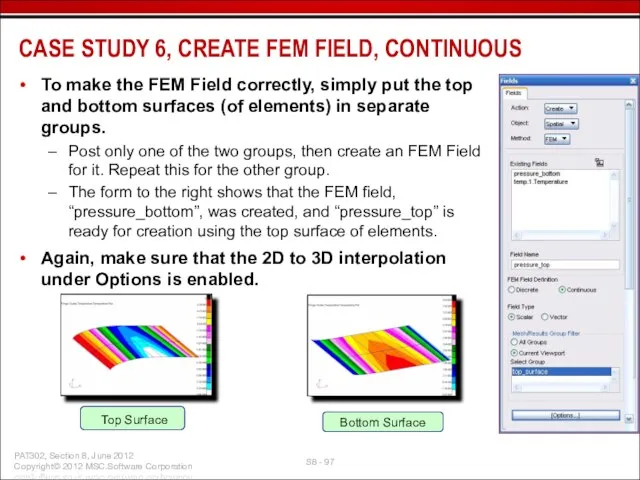
Слайд 97To make the FEM Field correctly, simply put the top and bottom
To make the FEM Field correctly, simply put the top and bottom
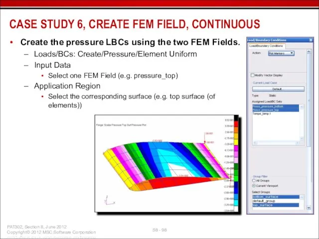
Слайд 98Create the pressure LBCs using the two FEM Fields.
Loads/BCs: Create/Pressure/Element Uniform
Input Data
Select
Create the pressure LBCs using the two FEM Fields.
Loads/BCs: Create/Pressure/Element Uniform
Input Data
Select
Слайд 99Perform Workshop 19 “Global/Local Modeling Using FEM Fields” in your exercise workbook.
EXERCISES
Perform Workshop 19 “Global/Local Modeling Using FEM Fields” in your exercise workbook.
EXERCISES

Слайд 101This type of field is used to create varying material properties using
This type of field is used to create varying material properties using
Слайд 102The number of variables selected determines whether a one‑, two‑, or three‑dimensional
The number of variables selected determines whether a one‑, two‑, or three‑dimensional
Слайд 103The top portion of the Tabular Input, [Options] form controls how many
The top portion of the Tabular Input, [Options] form controls how many
![The top portion of the Tabular Input, [Options] form controls how many](/_ipx/f_webp&q_80&fit_contain&s_1440x1080/imagesDir/jpg/378814/slide-102.jpg)
Слайд 104Material Properties/General allows the cross reference of any material property to any
Material Properties/General allows the cross reference of any material property to any
Слайд 105Material Property/Model Variable is intended for creating fields from user defined variables.
To
Material Property/Model Variable is intended for creating fields from user defined variables.
To
Слайд 106Model variables are single value parameters (constants).
The value can be specified either
Model variables are single value parameters (constants).
The value can be specified either
Слайд 107Create/Variable/Value has an additional option to subsequently create a Field.
If Create Referencing
Create/Variable/Value has an additional option to subsequently create a Field.
If Create Referencing

Слайд 109Stress vs.
Temperature and Strain
Create a single field that describes an Aluminum
Stress vs.
Temperature and Strain
Create a single field that describes an Aluminum
Слайд 110CASE STUDY 7, MATERIAL PROPERTY FIELD
To create the field, select Temperature
CASE STUDY 7, MATERIAL PROPERTY FIELD
To create the field, select Temperature
Слайд 111In [Options] the Extrapolation Option chosen does not affect the field evaluation
In [Options] the Extrapolation Option chosen does not affect the field evaluation
![In [Options] the Extrapolation Option chosen does not affect the field evaluation](/_ipx/f_webp&q_80&fit_contain&s_1440x1080/imagesDir/jpg/378814/slide-110.jpg)
Слайд 112In Materials, Input Properties there are two steps for making the nonlinear
In Materials, Input Properties there are two steps for making the nonlinear
Слайд 113Set the Constitutive Model to Nonlinear Elastic, and select the previously created
Set the Constitutive Model to Nonlinear Elastic, and select the previously created

Слайд 115Non Spatial, Real fields are used to create time or frequency dependent
Non Spatial, Real fields are used to create time or frequency dependent
Слайд 116Create non-spatial field
Real
Time
Map Function to Table
PCL Expression f(time)
FIELDS, NON SPATIAL/TABULAR INPUT
Create non-spatial field
Real
Time
Map Function to Table
PCL Expression f(time)
FIELDS, NON SPATIAL/TABULAR INPUT
Слайд 117Edit the columns to include two additional points (Time, Value)
FIELDS, NON SPATIAL/TABULAR
Edit the columns to include two additional points (Time, Value)
FIELDS, NON SPATIAL/TABULAR
Слайд 118FIELDS, NON SPATIAL/TABULAR INPUT
FIELDS, NON SPATIAL/TABULAR INPUT
Слайд 119FIELDS, NON SPATIAL/TABULAR INPUT
FIELDS, NON SPATIAL/TABULAR INPUT
 Сроки проведения: апрель- май 2011 года Участники: 30 общеобразовательных учреждений из 14 территорий Пермского края: г.Александровск
 Шаблон презентации (Краш-тест)
 Разбор пробного тестирования
 Презентация на тему История налогов
 Эти странные иностранцы
 Универсальная b2b
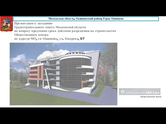 Заседание Градостроительного совета Московской области по вопросу продления срока действия разрешения на строительство центра
 Новогодние праздники позади… А мы всё чаще задумываемся о лете, о море…
 Ям К людям будете добры вы- Люди будут к вам добры!
 Детство Иисуса Христа
 Презентация на тему Кожно-мышечная чувствительность. Обоняние. Вкус
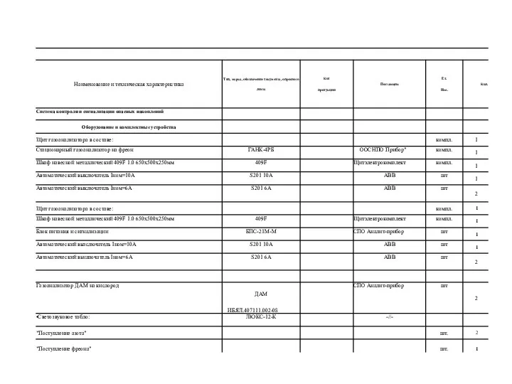 Система контроля и сигнализации опасных накоплений. Оборудование и комплектные устройства
 Экология чистоты с продуктами. Greenway Global
 Мастер-класс по изготовлению куклол-неразлучников
 Великая тайна воды
 Chill Map. Исследовательский проект
 Наследственное право РФ
 The Incredible Sun
  Офисный центр на улице Аврора 110, к.1
 Героическая оборона Москвы
 Название образовательного учреждения Творческий проект по технологии: « ТЕМА» Ученица 9 «А» класса Фамилия Имя Руководитель: Фами
 Презентация на тему Платон
 Вальпургеева ночь
 Образ Маши Мироновой в повести А.С.Пушкина «Капитанская дочка»
 Дифференциация с - ш в словах
 Презентация на тему Инновации в начальной школ
 Герои мультфильмов Уолта Диснея
 Презентация на тему Фоторяд "Дети войны"