Line broadening

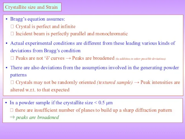
Crystallite size and Strain
Bragg’s equation assumes:
⮚ Crystal is perfect and infinite
⮚ Incident beam is perfectly parallel and monochromatic
Actual experimental conditions are different from these leading various kinds of deviations from Bragg’s condition
⮚ Peaks are not ‘δ’ curves → Peaks are broadened (in addition to other possible deviations)
There are also deviations from the assumptions involved in the generating powder patterns
⮚ Crystals may not be randomly oriented (textured sample) → Peak intensities are altered w.r.t. to that expected
In a powder sample if the crystallite size < 0.5 μm
⮚ there are insufficient number of planes to build up a sharp diffraction pattern
⇒ peaks are broadened

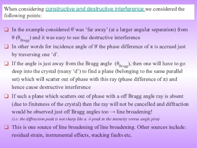
In the example considered θ’ was ‘far away’ (at a larger angular separation) from θ (θBragg) and it was easy to see the destructive interference
In other words for incidence angle of θ’ the phase difference of π is accrued just by traversing one ‘d’.
If the angle is just away from the Bragg angle (θBragg), then one will have to go deep into the crystal (many ‘d’) to find a plane (belonging to the same parallel set) which will scatter out of phase with this ray (phase difference of π) and hence cause destructive interference
If such a plane which scatters out of phase with a off Bragg angle ray is absent (due to finiteness of the crystal) then the ray will not be cancelled and diffraction would be observed just off Bragg angles too → line broadening!
(i.e. the diffraction peak is not sharp like a δ-peak in the intensity versus angle plot)
This is one source of line broadening of line broadening. Other sources include: residual strain, instrumental effects, stacking faults etc.
When considering constructive and destructive interference we considered the following points:

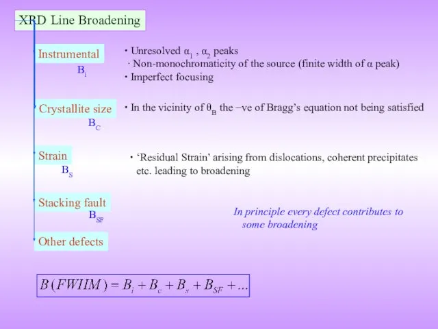
Instrumental
Crystallite size
Strain
Stacking fault
XRD Line Broadening
Other defects
Unresolved α1 , α2 peaks
∙ Non-monochromaticity of the source (finite width of α peak)
Imperfect focusing
In the vicinity of θB the −ve of Bragg’s equation not being satisfied
‘Residual Strain’ arising from dislocations, coherent precipitates etc. leading to broadening
In principle every defect contributes to some broadening
Bi
BC
BS
BSF

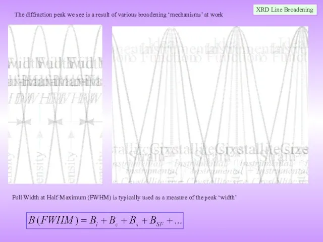
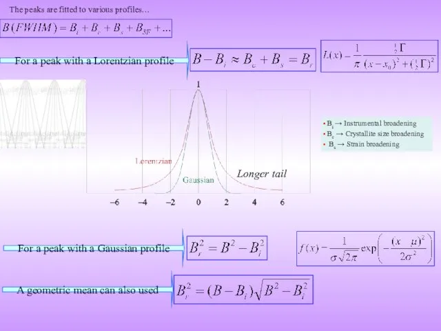
The diffraction peak we see is a result of various broadening ‘mechanisms’ at work
Full Width at Half-Maximum (FWHM) is typically used as a measure of the peak ‘width’
XRD Line Broadening

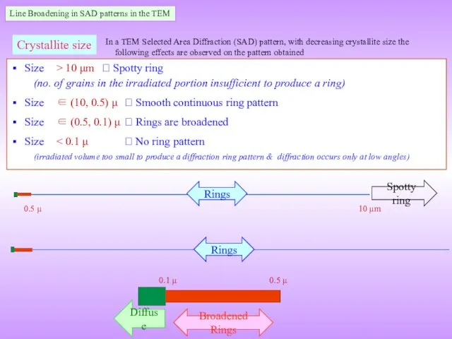
Crystallite size
Size > 10 μm ⮚ Spotty ring
(no. of grains in the irradiated portion insufficient to produce a ring)
Size ∈ (10, 0.5) μ ⮚ Smooth continuous ring pattern
Size ∈ (0.5, 0.1) μ ⮚ Rings are broadened
Size < 0.1 μ ⮚ No ring pattern
(irradiated volume too small to produce a diffraction ring pattern & diffraction occurs only at low angles)
Spotty ring
Rings
Broadened Rings
Diffuse
10 μm
0.5 μ
Rings
0.1 μ
0.5 μ
In a TEM Selected Area Diffraction (SAD) pattern, with decreasing crystallite size the following effects are observed on the pattern obtained
Line Broadening in SAD patterns in the TEM

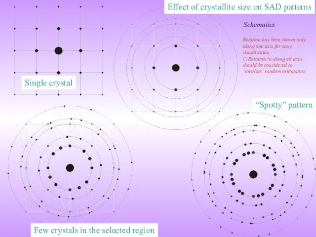
Effect of crystallite size on SAD patterns
Single crystal
“Spotty” pattern
Few crystals in the selected region
Schematics
Rotation has been shown only along one axis for easy visualization
⮚ Rotation in along all axes should be considered to ‘simulate’ random orientation

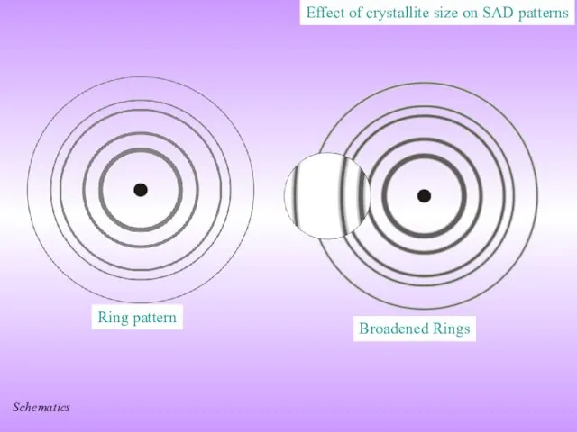
Effect of crystallite size on SAD patterns
Ring pattern
Broadened Rings
Schematics

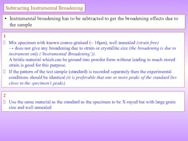
Subtracting Instrumental Broadening
Instrumental broadening has to be subtracted to get the broadening effects due to the sample
1
Mix specimen with known coarse-grained (~ 10μm), well annealed (strain free)
→ does not give any broadening due to strain or crystallite size (the broadening is due to instrument only (‘Instrumental Broadening’)).
A brittle material which can be ground into powder form without leading to much stored strain is good for this purpose.
If the pattern of the test sample (standard) is recorded separately then the experimental conditions should be identical (it is preferable that one or more peaks of the standard lies close to the specimen’s peaks)
2
Use the same material as the standard as the specimen to be X-rayed but with large grain size and well annealed

For a peak with a Lorentzian profile
For a peak with a Gaussian profile
A geometric mean can also used
Longer tail
The peaks are fitted to various profiles…
Bi → Instrumental broadening
Bc → Crystallite size broadening
Bs → Strain broadening

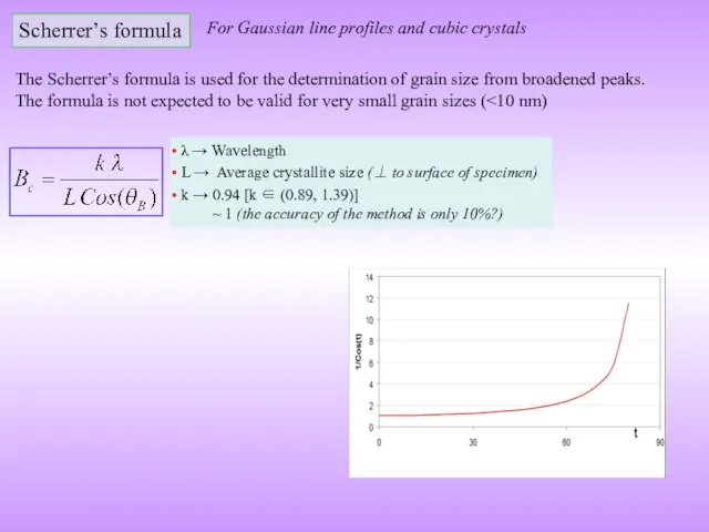
Scherrer’s formula
λ → Wavelength
L → Average crystallite size (⊥ to surface of specimen)
k → 0.94 [k ∈ (0.89, 1.39)]
~ 1 (the accuracy of the method is only 10%?)
For Gaussian line profiles and cubic crystals
The Scherrer’s formula is used for the determination of grain size from broadened peaks.
The formula is not expected to be valid for very small grain sizes (<10 nm)

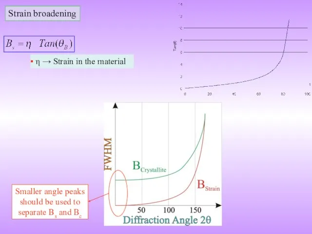
Strain broadening
η → Strain in the material
Smaller angle peaks
should be used to
separate Bs and Bc

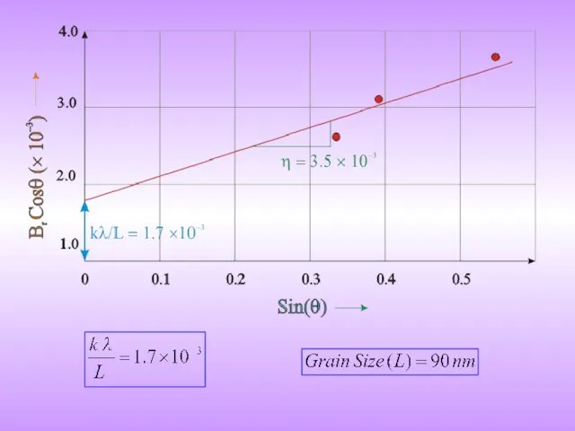
Separating crystallite size broadening and strain broadening
Plot of [Br Cosθ] vs [Sinθ]
Crystallite size broadening
Strain broadening

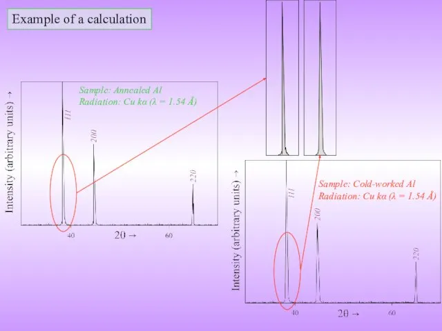
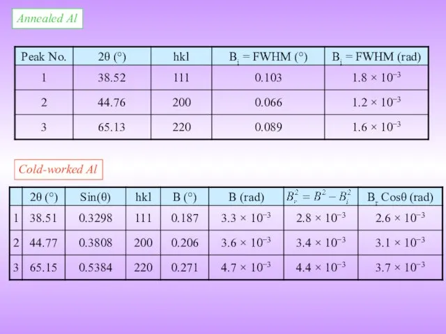
Example of a calculation
Sample: Annealed Al
Radiation: Cu kα (λ = 1.54 Å)
Sample: Cold-worked Al
Radiation: Cu kα (λ = 1.54 Å)

Annealed Al
Cold-worked Al