- Perfect Competition

Содержание
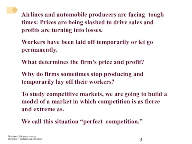
- 3. Airlines and automobile producers are facing tough times: Prices are being slashed to drive sales and
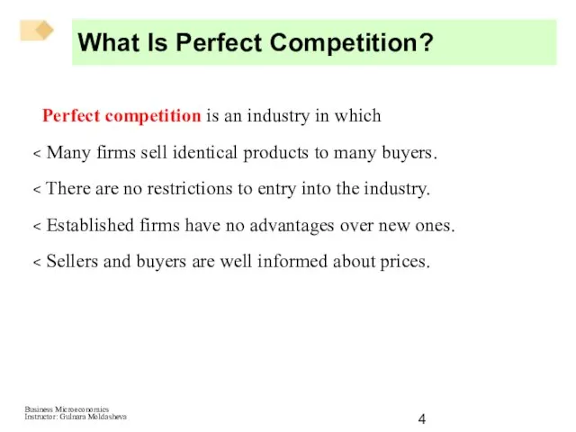
- 4. What Is Perfect Competition? Perfect competition is an industry in which Many firms sell identical products
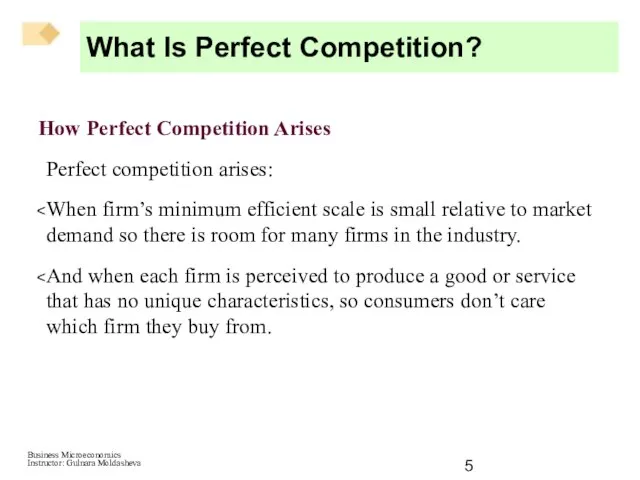
- 5. How Perfect Competition Arises Perfect competition arises: When firm’s minimum efficient scale is small relative to
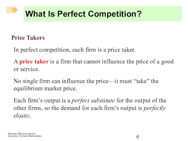
- 6. Price Takers In perfect competition, each firm is a price taker. A price taker is a
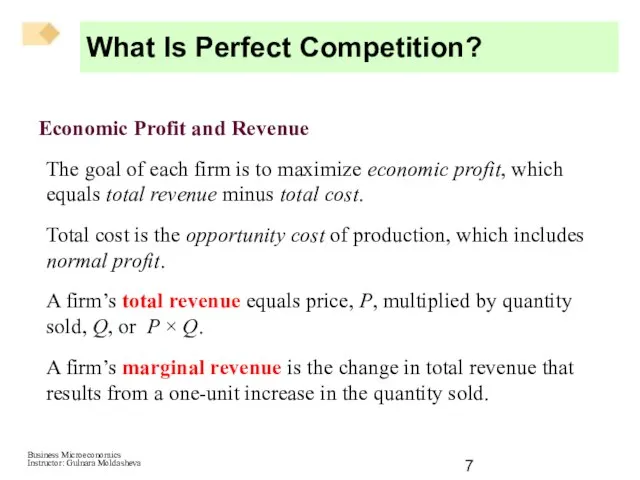
- 7. Economic Profit and Revenue The goal of each firm is to maximize economic profit, which equals
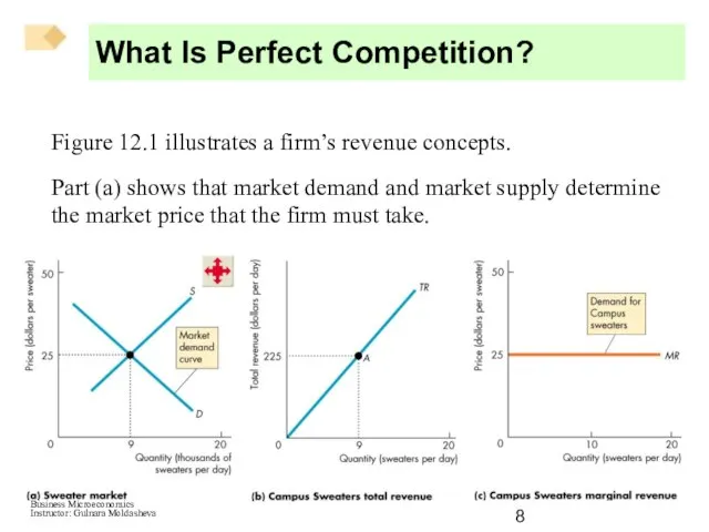
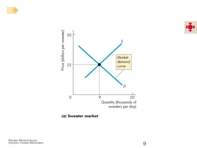
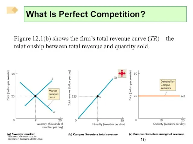
- 8. Figure 12.1 illustrates a firm’s revenue concepts. Part (a) shows that market demand and market supply
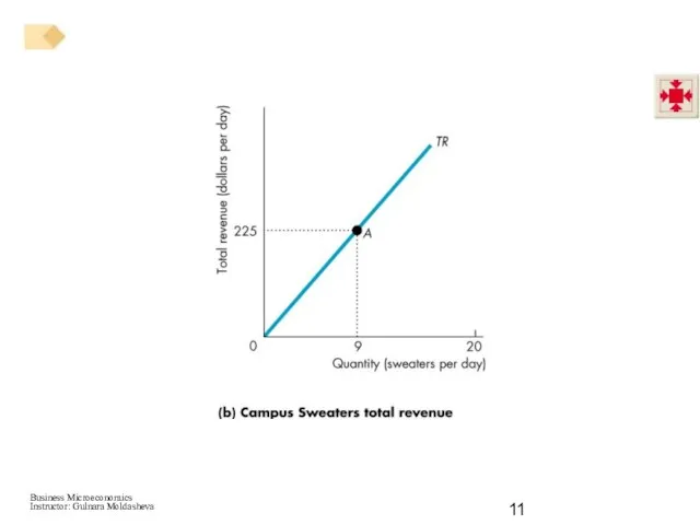
- 10. Figure 12.1(b) shows the firm’s total revenue curve (TR)—the relationship between total revenue and quantity sold.
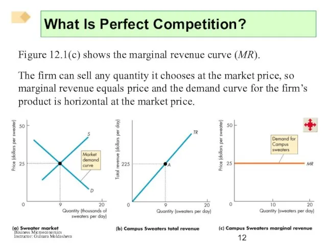
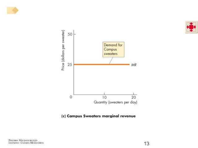
- 12. Figure 12.1(c) shows the marginal revenue curve (MR). The firm can sell any quantity it chooses
- 14. The demand for a firm’s product is perfectly elastic because one firm’s sweater is a perfect
- 15. A perfectly competitive firm’s goal is to make maximum economic profit, given the constraints it faces.
- 16. Profit-Maximizing Output A perfectly competitive firm chooses the output that maximizes its economic profit. One way
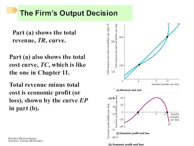
- 17. Part (a) shows the total revenue, TR, curve. Part (a) also shows the total cost curve,
- 19. At low output levels, the firm incurs an economic loss—it can’t cover its fixed costs. At
- 20. At high output levels, the firm again incurs an economic loss—now the firm faces steeply rising
- 21. Marginal Analysis and Supply Decision The firm can use marginal analysis to determine the profit-maximizing output.
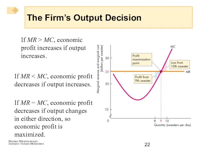
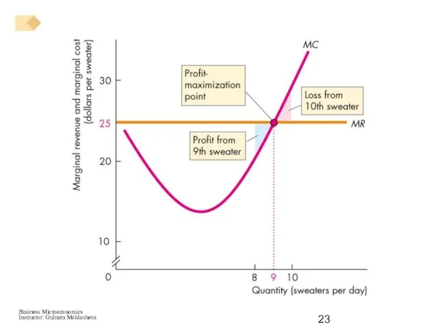
- 22. If MR > MC, economic profit increases if output increases. If MR If MR = MC,
- 24. Temporary Shutdown Decision If the firm makes an economic loss it must decide to exit the
- 25. Loss Comparison The firm’s loss equals total fixed cost (TFC) plus total variable cost (TVC) minus
- 26. A firm’s shutdown point is the price and quantity at which it is indifferent between producing
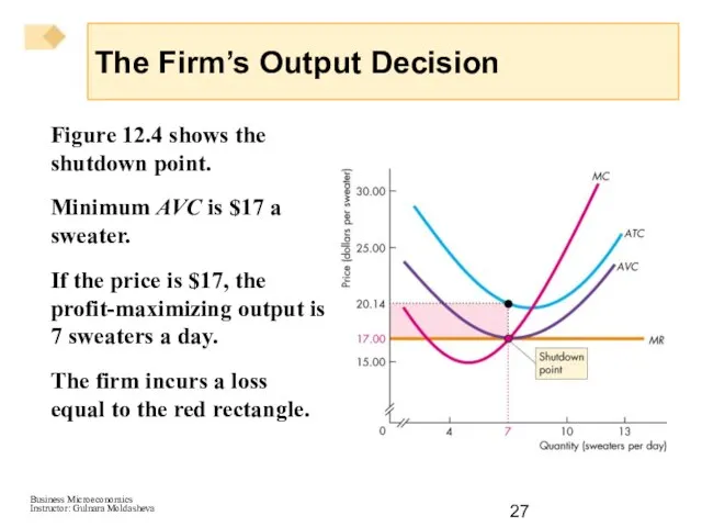
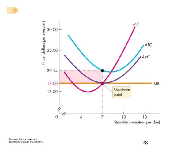
- 27. Figure 12.4 shows the shutdown point. Minimum AVC is $17 a sweater. If the price is
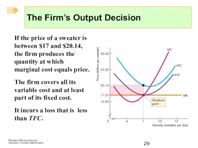
- 29. If the price of a sweater is between $17 and $20.14, the firm produces the quantity
- 30. The Firm’s Supply Curve A perfectly competitive firm’s supply curve shows how the firm’s profit-maximizing output
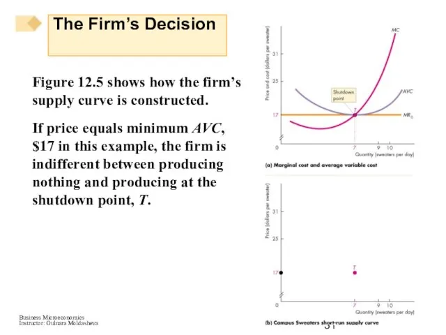
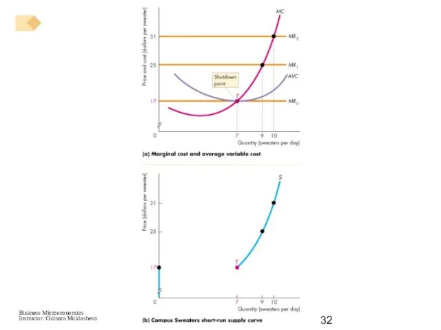
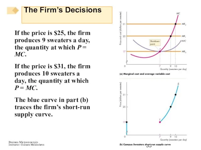
- 31. Figure 12.5 shows how the firm’s supply curve is constructed. If price equals minimum AVC, $17
- 33. If the price is $25, the firm produces 9 sweaters a day, the quantity at which
- 34. Market Supply in the Short Run The short-run market supply curve shows the quantity supplied by
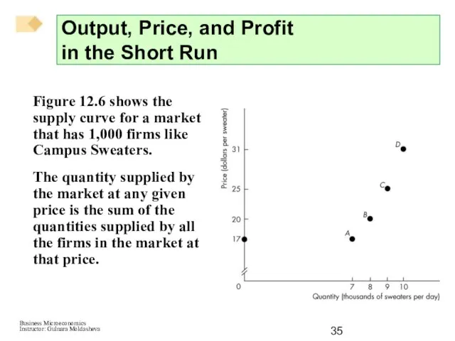
- 35. Figure 12.6 shows the supply curve for a market that has 1,000 firms like Campus Sweaters.
- 37. At a price equal to minimum AVC, the shutdown price, some firms will produce the shutdown
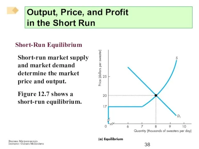
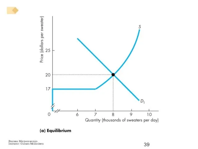
- 38. Short-Run Equilibrium Short-run market supply and market demand determine the market price and output. Figure 12.7
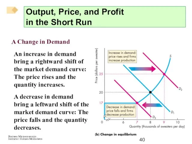
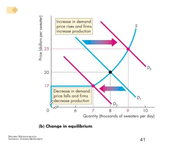
- 40. A Change in Demand An increase in demand bring a rightward shift of the market demand
- 42. Profits and Losses in the Short Run Maximum profit is not always a positive economic profit.
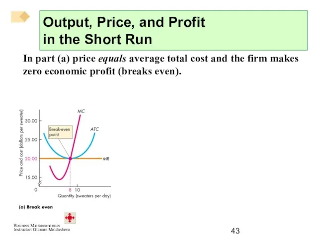
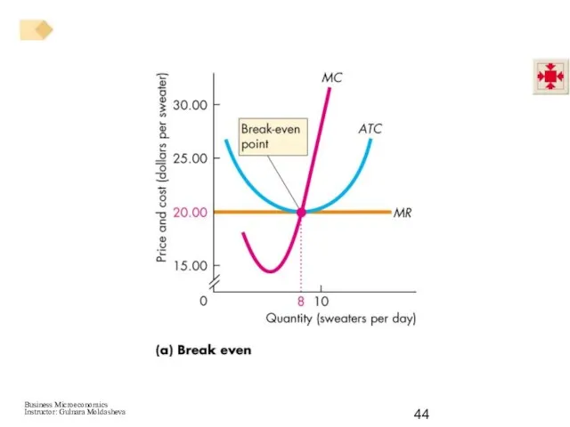
- 43. In part (a) price equals average total cost and the firm makes zero economic profit (breaks
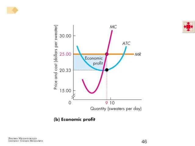
- 45. In part (b), price exceeds average total cost and the firm makes a positive economic profit.
- 47. In part (c) price is less than average total cost and the firm incurs an economic
- 49. In short-run equilibrium, a firm may make an economic profit, break even, or incur an economic
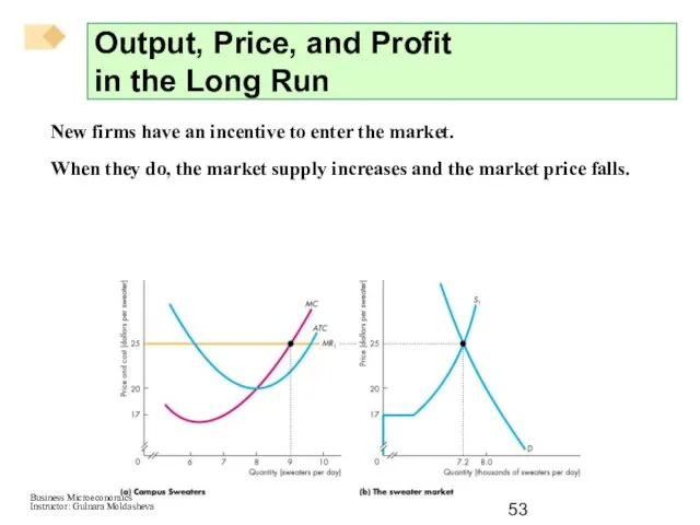
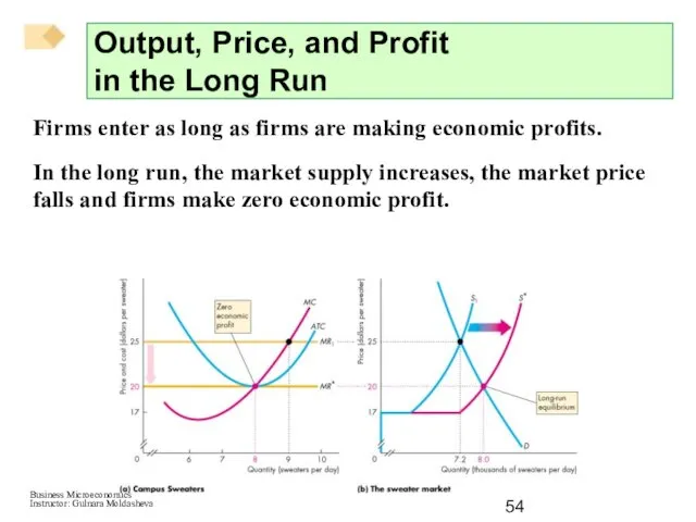
- 50. Entry and Exit New firms enter an industry in which existing firms make an economic profit.
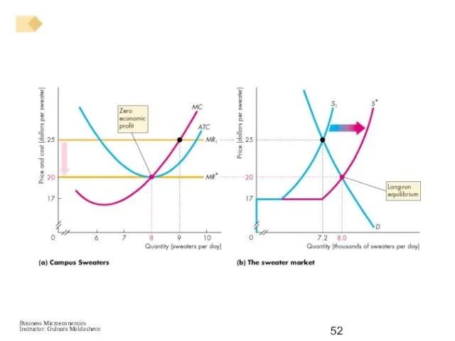
- 51. A Closer Look at Entry When the market price is $25 a sweater, firms in the
- 53. New firms have an incentive to enter the market. When they do, the market supply increases
- 54. Firms enter as long as firms are making economic profits. In the long run, the market
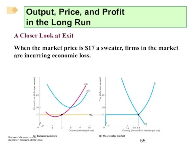
- 55. A Closer Look at Exit When the market price is $17 a sweater, firms in the
- 57. Firms have an incentive to exit the market. When they do, the market supply decreases and
- 58. Firms exit as long as firms are incurring economic losses. In the long run, the market
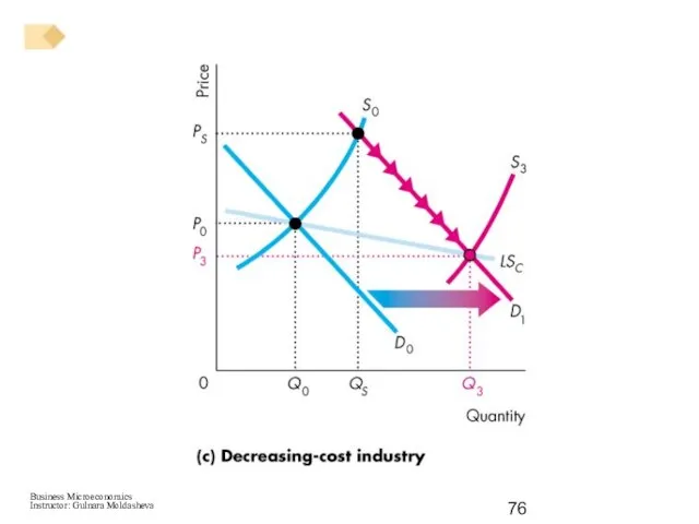
- 59. Changing Tastes and Advancing Technology A Permanent Change in Demand A decrease in demand shifts the
- 60. A decrease in demand shifts the market demand curve leftward. The market price falls, and each
- 62. The market price is now below each firm’s minimum average total cost, so firms incur economic
- 63. Economic losses induce some firms to exit in the long run, which decreases the market supply
- 64. As the price rises, the quantity produced by all firms continues to decrease as more firms
- 65. A new long-run equilibrium occurs when the price has risen to equal minimum average total cost.
- 66. The main difference between the initial and new long-run equilibrium is the number of firms in
- 67. A permanent increase in demand has the opposite effects to those just described and shown in
- 68. With a falling price, each firm decreases its output as it moves along its marginal cost
- 69. External Economics and Diseconomies The change in the long-run equilibrium price following a permanent change in
- 70. In the absence of external economies or external diseconomies, a firm’s costs remain constant as the
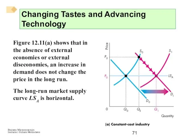
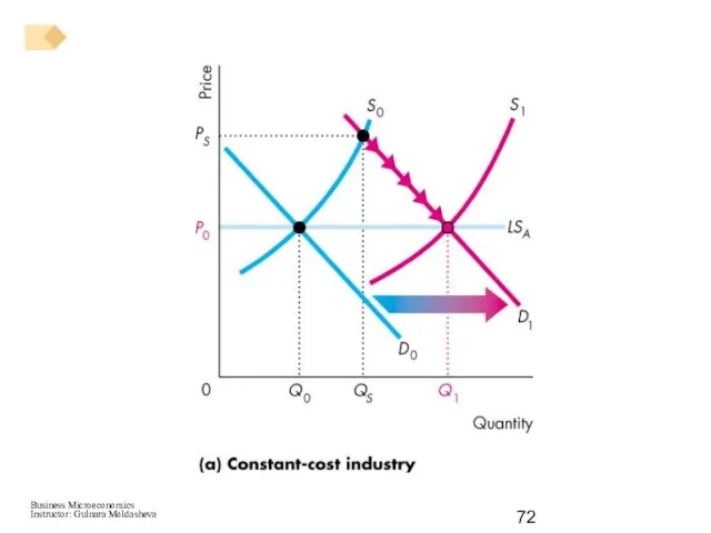
- 71. Figure 12.11(a) shows that in the absence of external economies or external diseconomies, an increase in
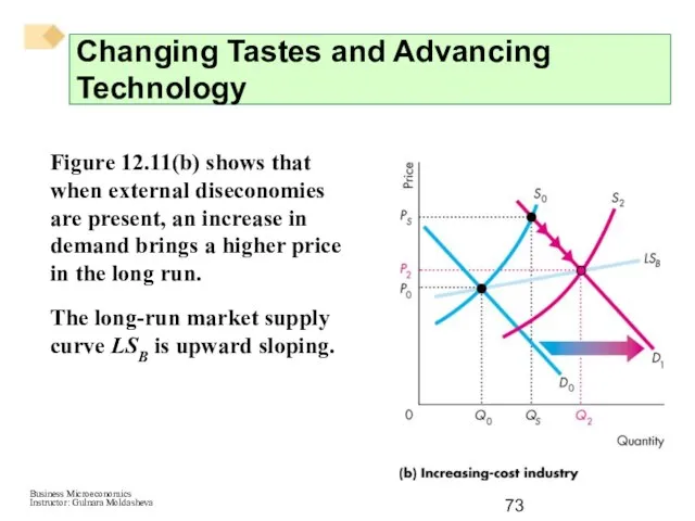
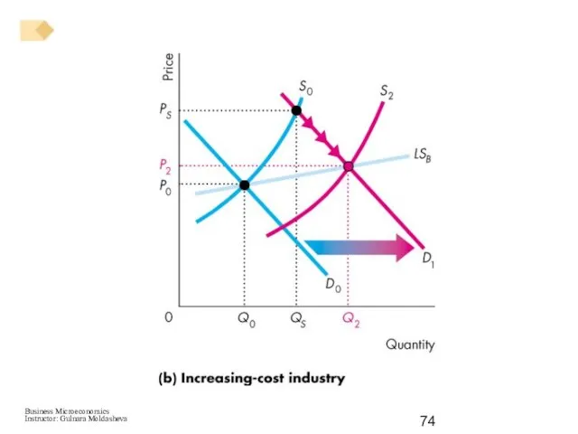
- 73. Figure 12.11(b) shows that when external diseconomies are present, an increase in demand brings a higher
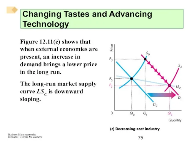
- 75. Figure 12.11(c) shows that when external economies are present, an increase in demand brings a lower
- 77. Technological Change New technologies are constantly discovered that lower costs. A new technology enables firms to
- 78. New-technology firms enter and old-technology firms either exit or adopt the new technology. Industry supply increases
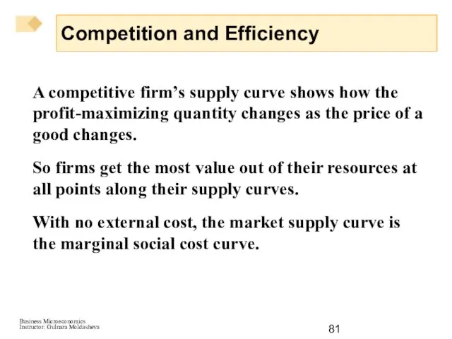
- 79. Competition and Efficiency Efficient Use of Resources Resources are used efficiently when no one can be
- 80. Choices, Equilibrium, and Efficiency We can describe an efficient use of resources in terms of the
- 81. A competitive firm’s supply curve shows how the profit-maximizing quantity changes as the price of a
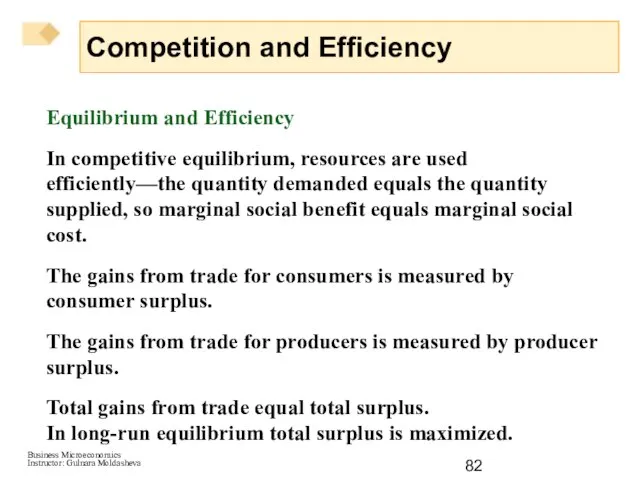
- 82. Equilibrium and Efficiency In competitive equilibrium, resources are used efficiently—the quantity demanded equals the quantity supplied,
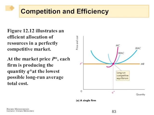
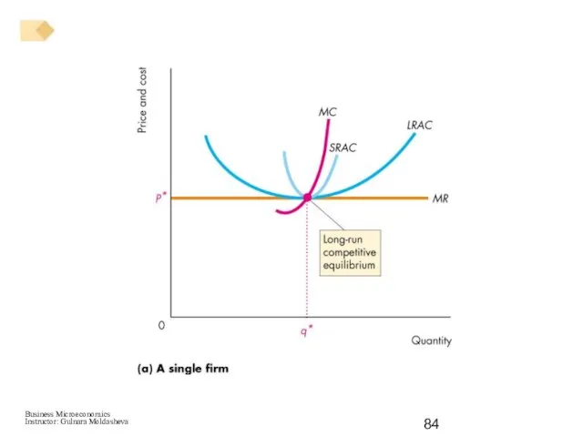
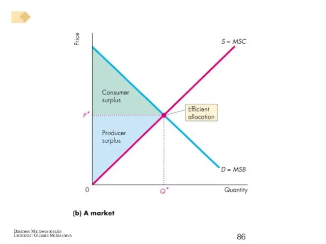
- 83. Figure 12.12 illustrates an efficient allocation of resources in a perfectly competitive market. At the market
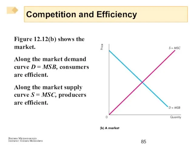
- 85. Figure 12.12(b) shows the market. Along the market demand curve D = MSB, consumers are efficient.
- 88. Скачать презентацию
Слайд 3Airlines and automobile producers are facing tough times: Prices are being slashed
Airlines and automobile producers are facing tough times: Prices are being slashed
Слайд 4What Is Perfect Competition?
Perfect competition is an industry in which
Many firms
What Is Perfect Competition?
Perfect competition is an industry in which
Many firms
Слайд 5How Perfect Competition Arises
Perfect competition arises:
When firm’s minimum efficient scale is small
How Perfect Competition Arises
Perfect competition arises:
When firm’s minimum efficient scale is small
Слайд 6Price Takers
In perfect competition, each firm is a price taker.
A price taker
Price Takers
In perfect competition, each firm is a price taker.
A price taker
Слайд 7Economic Profit and Revenue
The goal of each firm is to maximize economic
Economic Profit and Revenue
The goal of each firm is to maximize economic
Слайд 8Figure 12.1 illustrates a firm’s revenue concepts.
Part (a) shows that market demand
Figure 12.1 illustrates a firm’s revenue concepts.
Part (a) shows that market demand
Слайд 10Figure 12.1(b) shows the firm’s total revenue curve (TR)—the relationship between total
Figure 12.1(b) shows the firm’s total revenue curve (TR)—the relationship between total
Слайд 12Figure 12.1(c) shows the marginal revenue curve (MR).
The firm can sell any
Figure 12.1(c) shows the marginal revenue curve (MR).
The firm can sell any
Слайд 14The demand for a firm’s product is perfectly elastic because one firm’s
The demand for a firm’s product is perfectly elastic because one firm’s
Слайд 15A perfectly competitive firm’s goal is to make maximum economic profit, given
A perfectly competitive firm’s goal is to make maximum economic profit, given
Слайд 16Profit-Maximizing Output
A perfectly competitive firm chooses the output that maximizes its economic
Profit-Maximizing Output
A perfectly competitive firm chooses the output that maximizes its economic
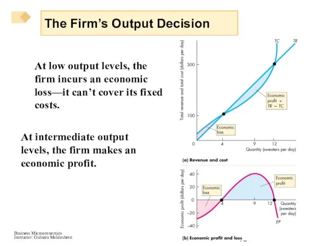
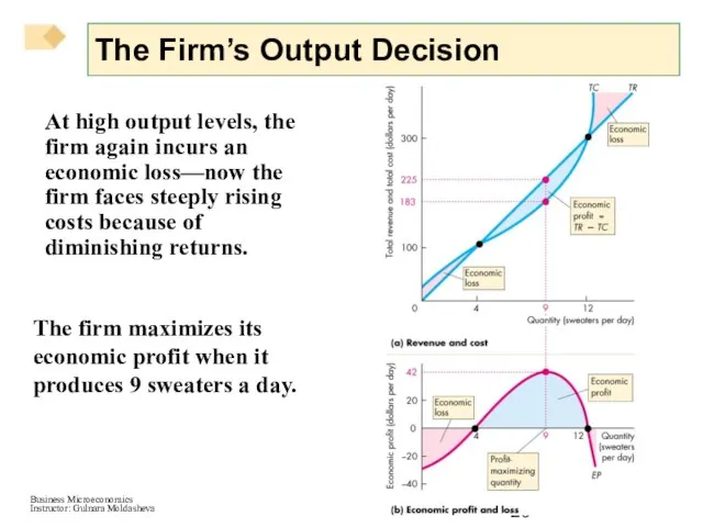
Слайд 17Part (a) shows the total revenue, TR, curve.
Part (a) also shows the
Part (a) shows the total revenue, TR, curve.
Part (a) also shows the
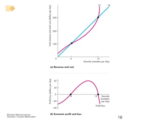
Слайд 19At low output levels, the firm incurs an economic loss—it can’t cover
At low output levels, the firm incurs an economic loss—it can’t cover
Слайд 20At high output levels, the firm again incurs an economic loss—now the
At high output levels, the firm again incurs an economic loss—now the
Слайд 21Marginal Analysis and Supply Decision
The firm can use marginal analysis to determine
Marginal Analysis and Supply Decision
The firm can use marginal analysis to determine
Слайд 22If MR > MC, economic profit increases if output increases.
If MR <
If MR > MC, economic profit increases if output increases.
If MR <
Слайд 24Temporary Shutdown Decision
If the firm makes an economic loss it must decide
Temporary Shutdown Decision
If the firm makes an economic loss it must decide
Слайд 25Loss Comparison
The firm’s loss equals total fixed cost (TFC) plus total variable
Loss Comparison
The firm’s loss equals total fixed cost (TFC) plus total variable
Слайд 26A firm’s shutdown point is the price and quantity at which it
A firm’s shutdown point is the price and quantity at which it
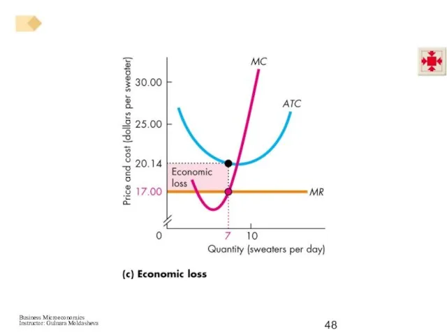
Слайд 27Figure 12.4 shows the shutdown point.
Minimum AVC is $17 a sweater.
If the
Figure 12.4 shows the shutdown point.
Minimum AVC is $17 a sweater.
If the
Слайд 29If the price of a sweater is between $17 and $20.14, the
If the price of a sweater is between $17 and $20.14, the
Слайд 30The Firm’s Supply Curve
A perfectly competitive firm’s supply curve shows how the
The Firm’s Supply Curve
A perfectly competitive firm’s supply curve shows how the

Слайд 31Figure 12.5 shows how the firm’s supply curve is constructed.
If price equals
Figure 12.5 shows how the firm’s supply curve is constructed.
If price equals
Слайд 33If the price is $25, the firm produces 9 sweaters a day,
If the price is $25, the firm produces 9 sweaters a day,
Слайд 34Market Supply in the Short Run
The short-run market supply curve shows the
Market Supply in the Short Run
The short-run market supply curve shows the
Слайд 35Figure 12.6 shows the supply curve for a market that has 1,000
Figure 12.6 shows the supply curve for a market that has 1,000
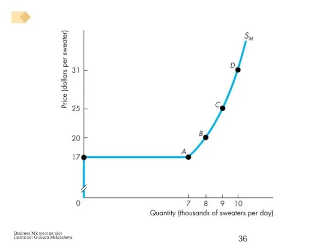
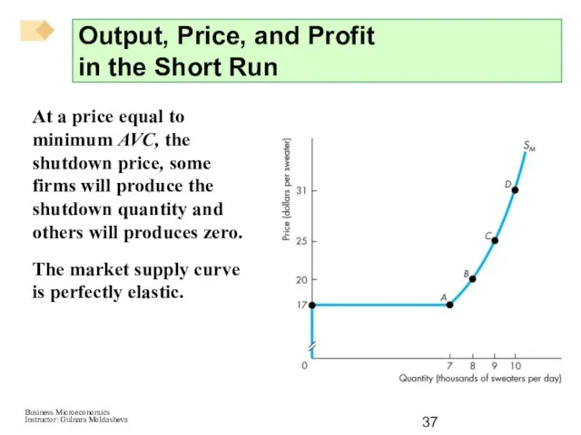
Слайд 37At a price equal to minimum AVC, the shutdown price, some firms
At a price equal to minimum AVC, the shutdown price, some firms
Слайд 38Short-Run Equilibrium
Short-run market supply and market demand determine the market price and
Short-Run Equilibrium
Short-run market supply and market demand determine the market price and
Слайд 40A Change in Demand
An increase in demand bring a rightward shift
A Change in Demand
An increase in demand bring a rightward shift
Слайд 42Profits and Losses in the Short Run
Maximum profit is not always a
Profits and Losses in the Short Run
Maximum profit is not always a
Слайд 43In part (a) price equals average total cost and the firm makes
In part (a) price equals average total cost and the firm makes
Слайд 45In part (b), price exceeds average total cost and the firm makes
In part (b), price exceeds average total cost and the firm makes

Слайд 47In part (c) price is less than average total cost and the
In part (c) price is less than average total cost and the
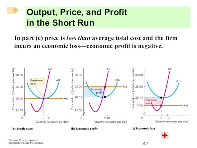
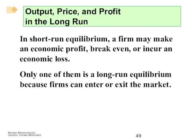
Слайд 49In short-run equilibrium, a firm may make an economic profit, break even,
In short-run equilibrium, a firm may make an economic profit, break even,
Слайд 50Entry and Exit
New firms enter an industry in which existing firms make
Entry and Exit
New firms enter an industry in which existing firms make
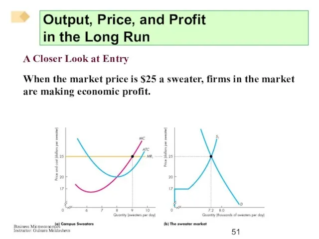
Слайд 51A Closer Look at Entry
When the market price is $25 a sweater,
A Closer Look at Entry
When the market price is $25 a sweater,
Слайд 53New firms have an incentive to enter the market.
When they do, the
New firms have an incentive to enter the market.
When they do, the
Слайд 54Firms enter as long as firms are making economic profits.
In the
Firms enter as long as firms are making economic profits.
In the
Слайд 55A Closer Look at Exit
When the market price is $17 a sweater,
A Closer Look at Exit
When the market price is $17 a sweater,
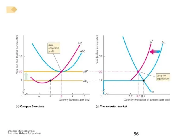
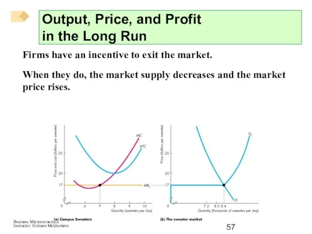
Слайд 57Firms have an incentive to exit the market.
When they do, the market
Firms have an incentive to exit the market.
When they do, the market
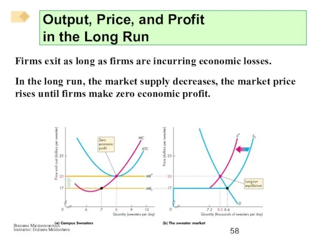
Слайд 58Firms exit as long as firms are incurring economic losses.
In the
Firms exit as long as firms are incurring economic losses.
In the
Слайд 59Changing Tastes and Advancing Technology
A Permanent Change in Demand
A decrease in demand
Changing Tastes and Advancing Technology
A Permanent Change in Demand
A decrease in demand
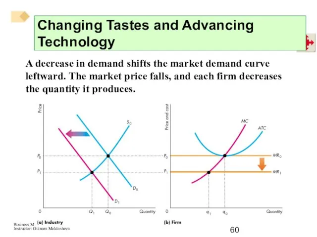
Слайд 60A decrease in demand shifts the market demand curve leftward. The market
A decrease in demand shifts the market demand curve leftward. The market
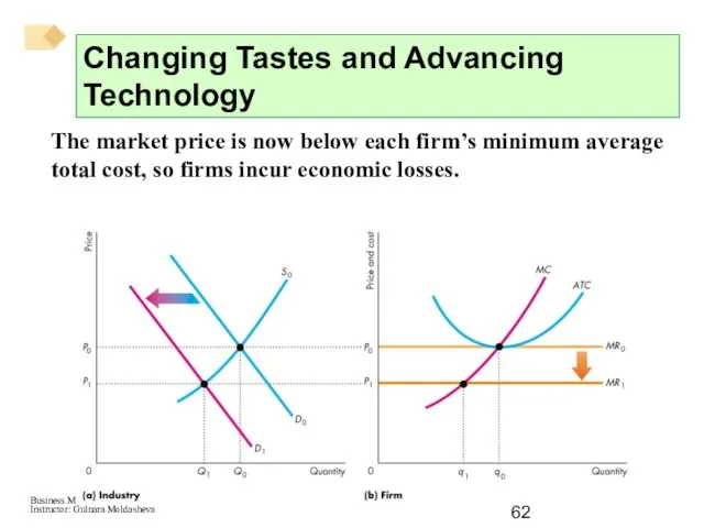
Слайд 62The market price is now below each firm’s minimum average total cost,
The market price is now below each firm’s minimum average total cost,
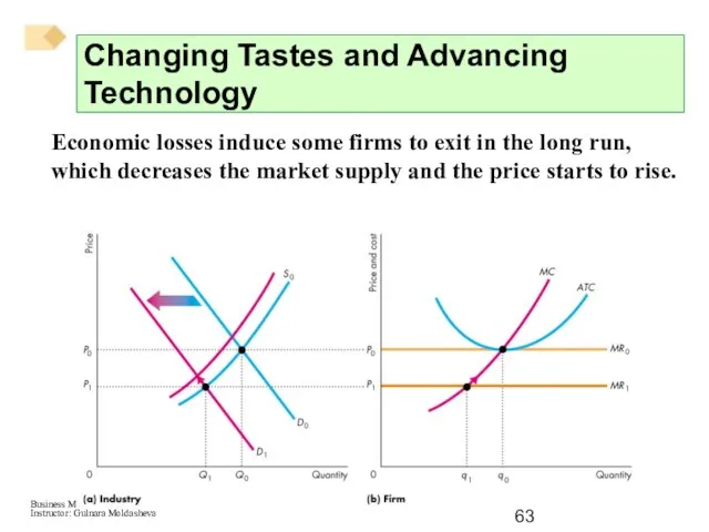
Слайд 63Economic losses induce some firms to exit in the long run, which
Economic losses induce some firms to exit in the long run, which
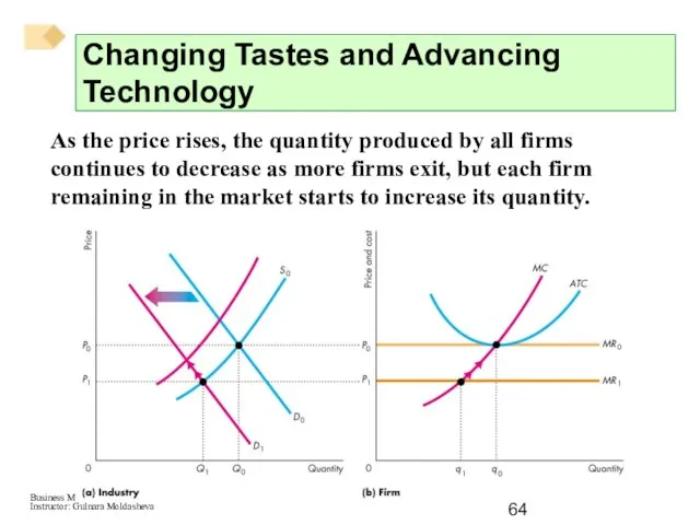
Слайд 64As the price rises, the quantity produced by all firms continues to
As the price rises, the quantity produced by all firms continues to
Слайд 65A new long-run equilibrium occurs when the price has risen to equal
A new long-run equilibrium occurs when the price has risen to equal
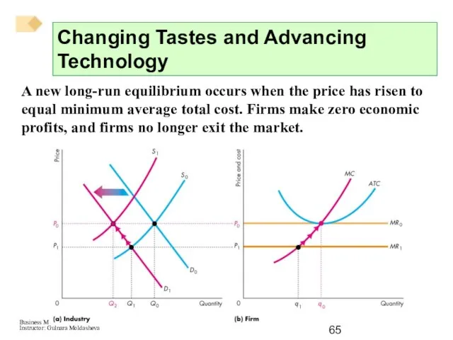
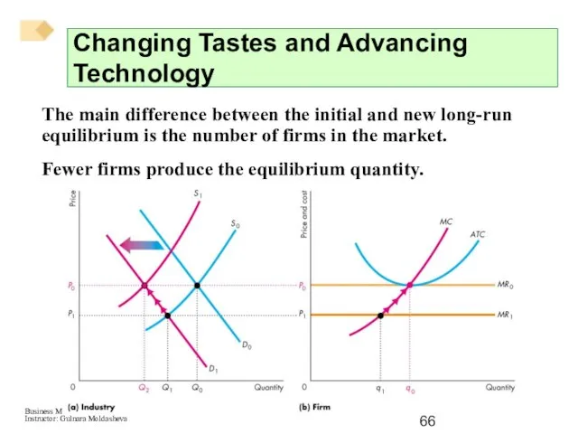
Слайд 66The main difference between the initial and new long-run equilibrium is the
The main difference between the initial and new long-run equilibrium is the
Слайд 67A permanent increase in demand has the opposite effects to those just
A permanent increase in demand has the opposite effects to those just
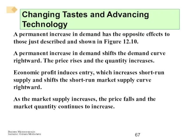
Слайд 68With a falling price, each firm decreases its output as it moves
With a falling price, each firm decreases its output as it moves
Слайд 69External Economics and Diseconomies
The change in the long-run equilibrium price following a
External Economics and Diseconomies
The change in the long-run equilibrium price following a
Слайд 70In the absence of external economies or external diseconomies, a firm’s costs
In the absence of external economies or external diseconomies, a firm’s costs
Слайд 71Figure 12.11(a) shows that in the absence of external economies or external
Figure 12.11(a) shows that in the absence of external economies or external
Слайд 73Figure 12.11(b) shows that when external diseconomies are present, an increase in
Figure 12.11(b) shows that when external diseconomies are present, an increase in
Слайд 75Figure 12.11(c) shows that when external economies are present, an increase in
Figure 12.11(c) shows that when external economies are present, an increase in
Слайд 77Technological Change
New technologies are constantly discovered that lower costs.
A new technology enables
Technological Change
New technologies are constantly discovered that lower costs.
A new technology enables

Слайд 78New-technology firms enter and old-technology firms either exit or adopt the new
New-technology firms enter and old-technology firms either exit or adopt the new
Слайд 79Competition and Efficiency
Efficient Use of Resources
Resources are used efficiently when no one
Competition and Efficiency
Efficient Use of Resources
Resources are used efficiently when no one
Слайд 80Choices, Equilibrium, and Efficiency
We can describe an efficient use of resources in
Choices, Equilibrium, and Efficiency
We can describe an efficient use of resources in
Слайд 81A competitive firm’s supply curve shows how the profit-maximizing quantity changes as
A competitive firm’s supply curve shows how the profit-maximizing quantity changes as
Слайд 82Equilibrium and Efficiency
In competitive equilibrium, resources are used efficiently—the quantity demanded equals
Equilibrium and Efficiency
In competitive equilibrium, resources are used efficiently—the quantity demanded equals
Слайд 83Figure 12.12 illustrates an efficient allocation of resources in a perfectly competitive
Figure 12.12 illustrates an efficient allocation of resources in a perfectly competitive
Слайд 85Figure 12.12(b) shows the market.
Along the market demand curve D = MSB,
Figure 12.12(b) shows the market.
Along the market demand curve D = MSB,
 Презентация на тему Социальный портрет молодежи 8/24/16
  Презентация-ООО-ХимСталь
 Грамоты благодарности родителям за хорошее воспитание детей
 Языковой центр Top Way Language Center
 Портфолио Карпенко Анастасии
 Рисуночный тест Н.Г. Хитровой
 Аэродинамика тепловых установок
 Цифровое телевидение и инновации
 Дом как отражение личности
 Великие изобретения человечества
 Глаз. Особенности зрения
 Презентация на тему Создание надежной системы безопасности, сбалансированной по критерию безопасность-стоимость
  Кафедра таможенного дела Магистерская диссертация Эффективность таможенно-тарифной политики в создании безбарьерной внешнетор
 Пенсионная реформа 2015 года
 Толерантность – дорога к миру
 Технология приготовления сложных горячих соусов
 Звонят колокола в память о растерзанной душе Убеженского храма (вечер-экскурс в историю Михайло-Архангельской церкви станицы Убе
 Презентация на тему Демографическая проблема
  Лидер ЕДД: Прядезникова Варя
 Пиво, напитки, энергетические коктейли
 Характеристика отдельных видов транспорта
 Лого заголовок
 Восточные походы Александра Македонского
 Групповая динамика в команде разработчиков Игорь Лужанский
 Сложение чисел с помощью координатной прямой
 Панно Корзина с цветами
 Межрегиональный гуманитарный научный комитет им. К.П. Победоносцева
 "Обучение жизненно важным навыкам"