- Demand

Содержание
- 2. Properties of Demand Functions Comparative statics analysis of ordinary demand functions -- the study of how
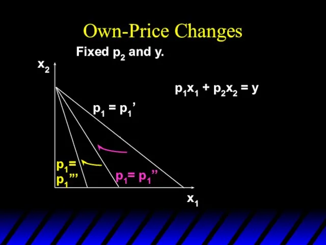
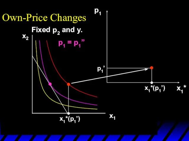
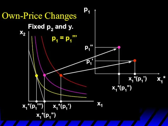
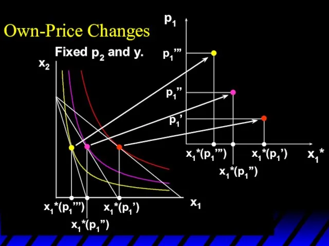
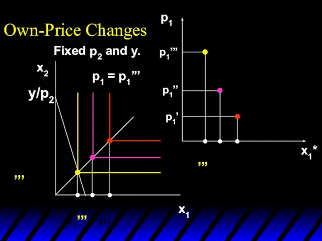
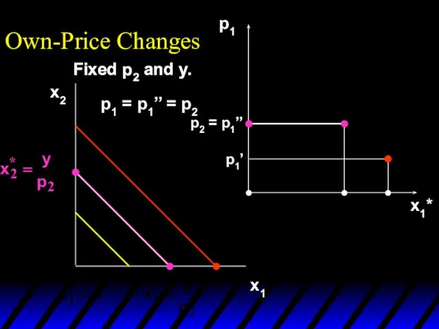
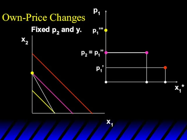
- 3. Own-Price Changes How does x1*(p1,p2,y) change as p1 changes, holding p2 and y constant? Suppose only
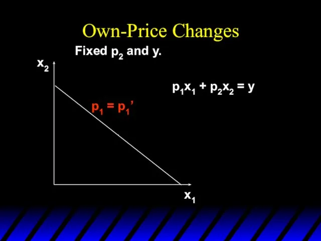
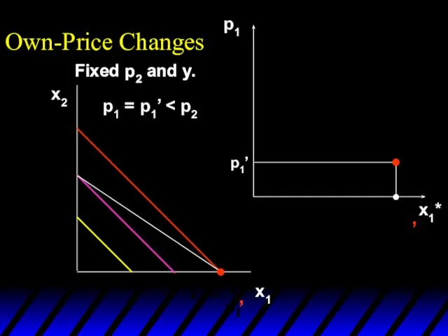
- 4. x1 x2 p1 = p1’ Fixed p2 and y. p1x1 + p2x2 = y Own-Price Changes
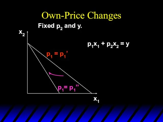
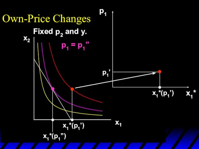
- 5. Own-Price Changes x1 x2 p1= p1’’ p1 = p1’ Fixed p2 and y. p1x1 + p2x2
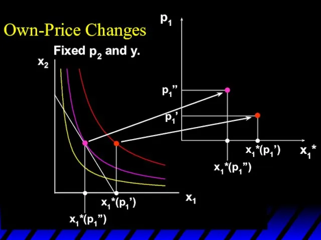
- 6. Own-Price Changes x1 x2 p1= p1’’ p1= p1’’’ Fixed p2 and y. p1 = p1’ p1x1
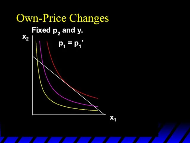
- 7. p1 = p1’ Own-Price Changes Fixed p2 and y.
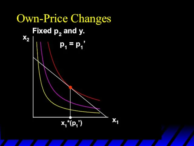
- 8. x1*(p1’) Own-Price Changes p1 = p1’ Fixed p2 and y.
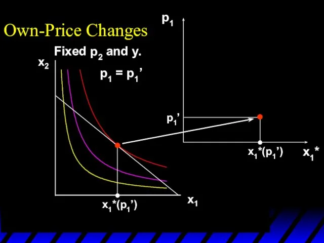
- 9. x1*(p1’) p1 x1*(p1’) p1’ x1* Own-Price Changes Fixed p2 and y. p1 = p1’
- 10. x1*(p1’) p1 x1*(p1’) p1’ p1 = p1’’ x1* Own-Price Changes Fixed p2 and y.
- 11. x1*(p1’) x1*(p1’’) p1 x1*(p1’) p1’ p1 = p1’’ x1* Own-Price Changes Fixed p2 and y.
- 12. x1*(p1’) x1*(p1’’) p1 x1*(p1’) x1*(p1’’) p1’ p1’’ x1* Own-Price Changes Fixed p2 and y.
- 13. x1*(p1’) x1*(p1’’) p1 x1*(p1’) x1*(p1’’) p1’ p1’’ p1 = p1’’’ x1* Own-Price Changes Fixed p2 and
- 14. x1*(p1’’’) x1*(p1’) x1*(p1’’) p1 x1*(p1’) x1*(p1’’) p1’ p1’’ p1 = p1’’’ x1* Own-Price Changes Fixed p2
- 15. x1*(p1’’’) x1*(p1’) x1*(p1’’) p1 x1*(p1’) x1*(p1’’’) x1*(p1’’) p1’ p1’’ p1’’’ x1* Own-Price Changes Fixed p2 and
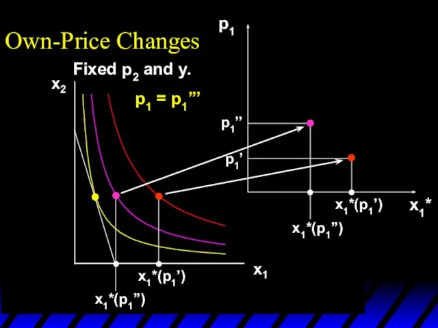
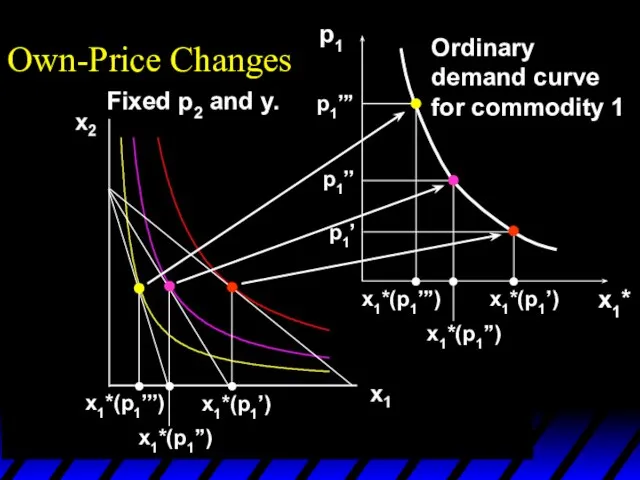
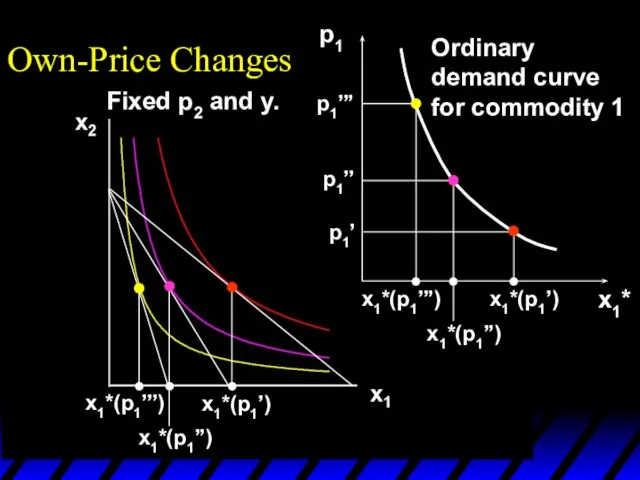
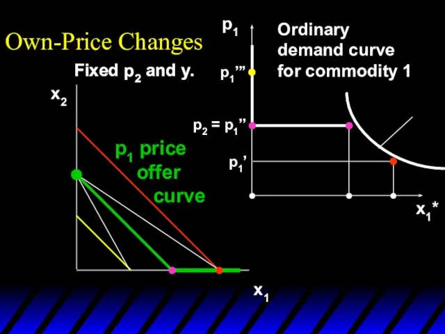
- 16. x1*(p1’’’) x1*(p1’) x1*(p1’’) p1 x1*(p1’) x1*(p1’’’) x1*(p1’’) p1’ p1’’ p1’’’ x1* Own-Price Changes Ordinary demand curve
- 17. x1*(p1’’’) x1*(p1’) x1*(p1’’) p1 x1*(p1’) x1*(p1’’’) x1*(p1’’) p1’ p1’’ p1’’’ x1* Own-Price Changes Ordinary demand curve
- 18. x1*(p1’’’) x1*(p1’) x1*(p1’’) p1 x1*(p1’) x1*(p1’’’) x1*(p1’’) p1’ p1’’ p1’’’ x1* Own-Price Changes Ordinary demand curve
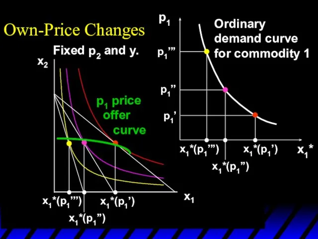
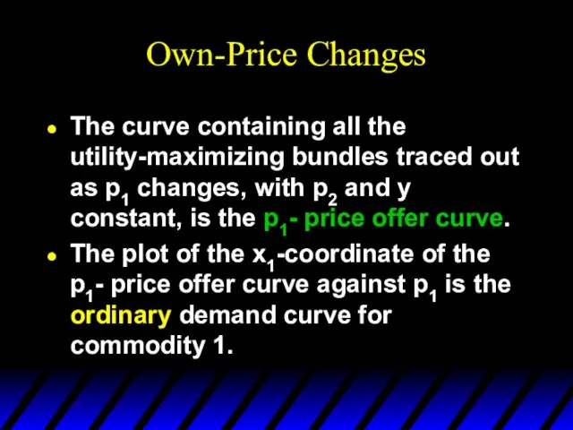
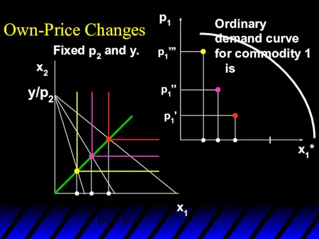
- 19. Own-Price Changes The curve containing all the utility-maximizing bundles traced out as p1 changes, with p2
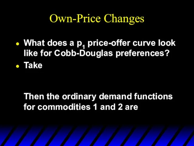
- 20. Own-Price Changes What does a p1 price-offer curve look like for Cobb-Douglas preferences?
- 21. Own-Price Changes What does a p1 price-offer curve look like for Cobb-Douglas preferences? Take Then the
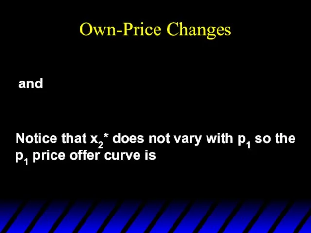
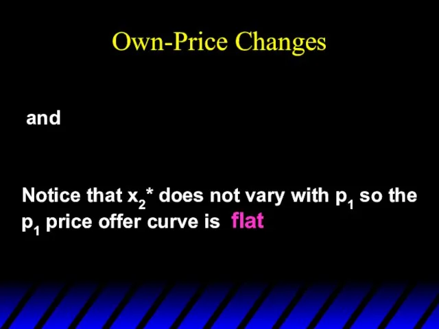
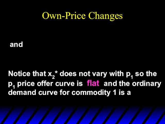
- 22. Own-Price Changes and Notice that x2* does not vary with p1 so the p1 price offer
- 23. Own-Price Changes and Notice that x2* does not vary with p1 so the p1 price offer
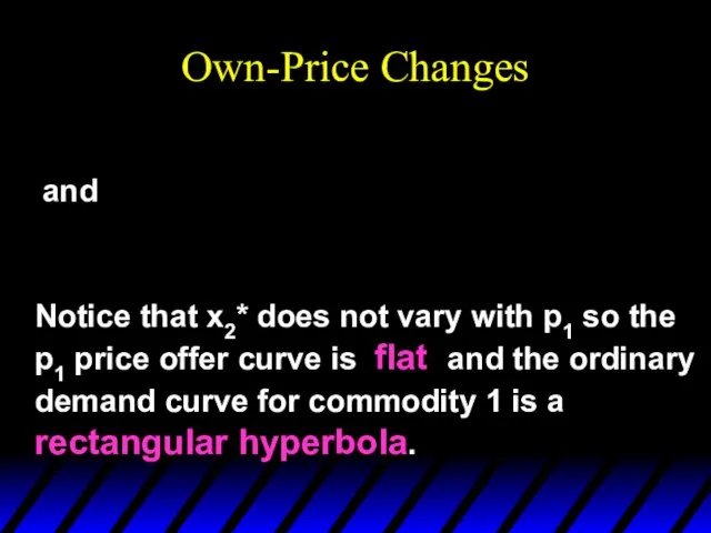
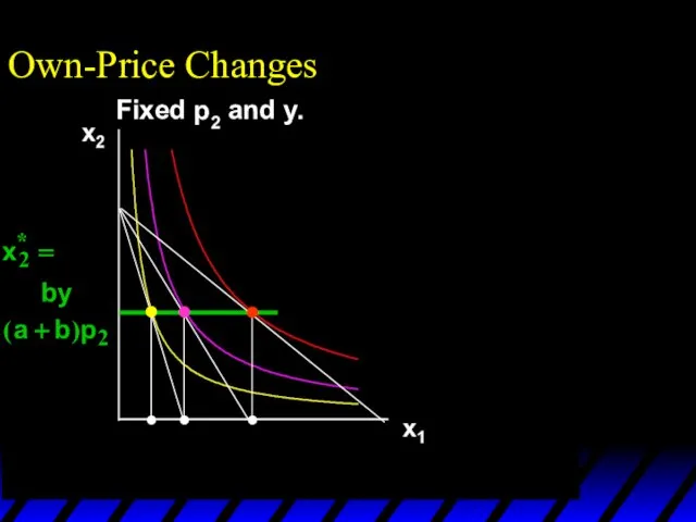
- 24. Own-Price Changes and Notice that x2* does not vary with p1 so the p1 price offer
- 25. Own-Price Changes and Notice that x2* does not vary with p1 so the p1 price offer
- 26. x1*(p1’’’) x1*(p1’) x1*(p1’’) Own-Price Changes Fixed p2 and y.
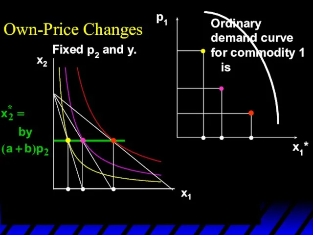
- 27. x1*(p1’’’) x1*(p1’) x1*(p1’’) p1 x1* Own-Price Changes Ordinary demand curve for commodity 1 is Fixed p2
- 28. Own-Price Changes What does a p1 price-offer curve look like for a perfect-complements utility function?
- 29. Own-Price Changes What does a p1 price-offer curve look like for a perfect-complements utility function? Then
- 30. Own-Price Changes
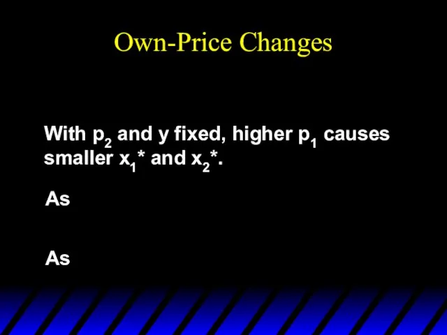
- 31. Own-Price Changes With p2 and y fixed, higher p1 causes smaller x1* and x2*.
- 32. Own-Price Changes With p2 and y fixed, higher p1 causes smaller x1* and x2*. As
- 33. Own-Price Changes With p2 and y fixed, higher p1 causes smaller x1* and x2*. As As
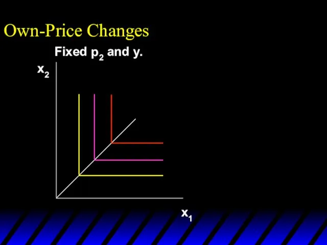
- 34. Fixed p2 and y. Own-Price Changes x1 x2
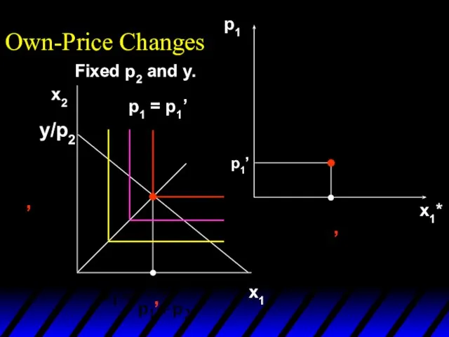
- 35. p1 x1* Fixed p2 and y. Own-Price Changes x1 x2 p1’ ’ p1 = p1’ ’
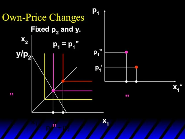
- 36. p1 x1* Fixed p2 and y. Own-Price Changes x1 x2 p1’ p1’’ p1 = p1’’ ’’
- 37. p1 x1* Fixed p2 and y. Own-Price Changes x1 x2 p1’ p1’’ p1’’’ p1 = p1’’’
- 38. p1 x1* Ordinary demand curve for commodity 1 is Fixed p2 and y. Own-Price Changes x1
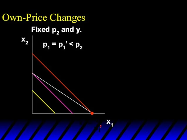
- 39. Own-Price Changes What does a p1 price-offer curve look like for a perfect-substitutes utility function? Then
- 40. Own-Price Changes and
- 41. Fixed p2 and y. Own-Price Changes x2 x1 Fixed p2 and y. p1 = p1’ ’
- 42. Fixed p2 and y. Own-Price Changes x2 x1 p1 x1* Fixed p2 and y. p1’ p1
- 43. Fixed p2 and y. Own-Price Changes x2 x1 p1 x1* Fixed p2 and y. p1’ p1
- 44. Fixed p2 and y. Own-Price Changes x2 x1 p1 x1* Fixed p2 and y. p1’ p1
- 45. Fixed p2 and y. Own-Price Changes x2 x1 p1 x1* Fixed p2 and y. p1’ p1
- 46. Fixed p2 and y. Own-Price Changes x2 x1 p1 x1* Fixed p2 and y. p1’ p1
- 47. Fixed p2 and y. Own-Price Changes x2 x1 p1 x1* Fixed p2 and y. p1’ p1’’’
- 48. Fixed p2 and y. Own-Price Changes x2 x1 p1 x1* Fixed p2 and y. p1’ p2
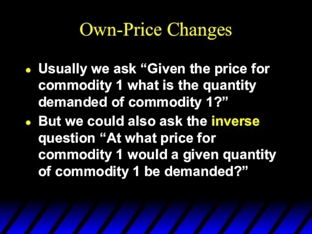
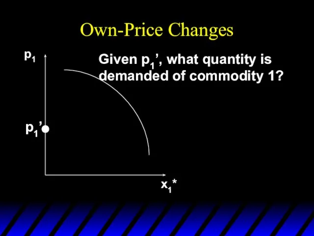
- 49. Own-Price Changes Usually we ask “Given the price for commodity 1 what is the quantity demanded
- 50. Own-Price Changes p1 x1* p1’ Given p1’, what quantity is demanded of commodity 1?
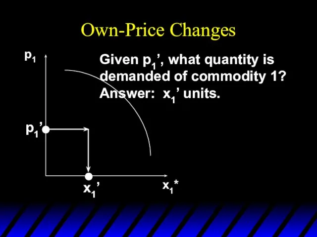
- 51. Own-Price Changes p1 x1* p1’ Given p1’, what quantity is demanded of commodity 1? Answer: x1’
- 52. Own-Price Changes p1 x1* x1’ Given p1’, what quantity is demanded of commodity 1? Answer: x1’
- 53. Own-Price Changes p1 x1* p1’ x1’ Given p1’, what quantity is demanded of commodity 1? Answer:
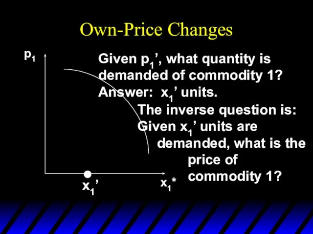
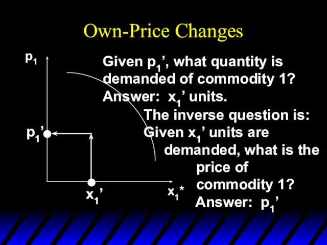
- 54. Own-Price Changes Taking quantity demanded as given and then asking what must be price describes the
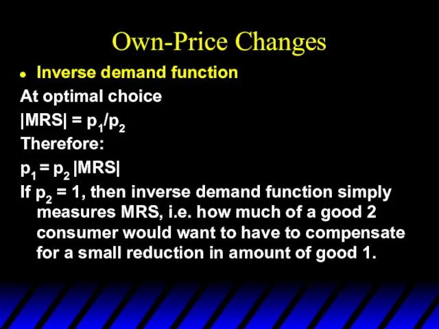
- 55. Own-Price Changes Inverse demand function At optimal choice |MRS| = p1/p2 Therefore: p1 = p2 |MRS|
- 56. Own-Price Changes Inverse demand function If good 2 is money, then MRS (and inverse demand function)
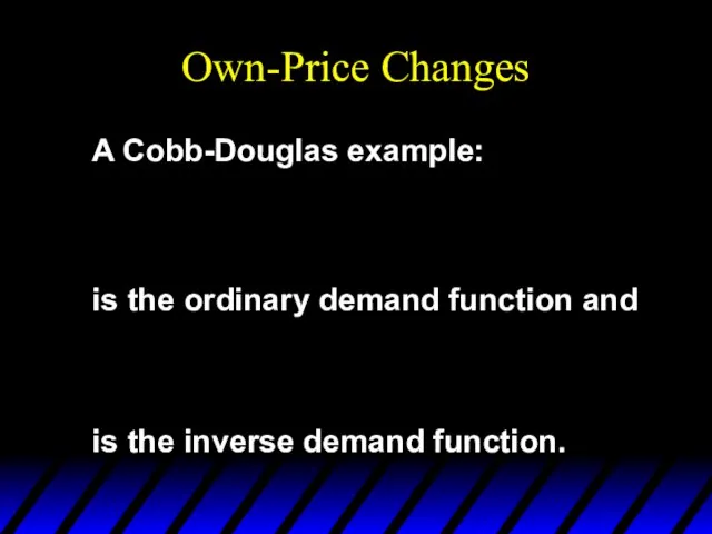
- 57. Own-Price Changes A Cobb-Douglas example: is the ordinary demand function and is the inverse demand function.
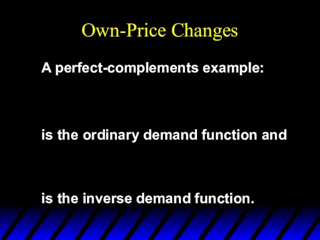
- 58. Own-Price Changes A perfect-complements example: is the ordinary demand function and is the inverse demand function.
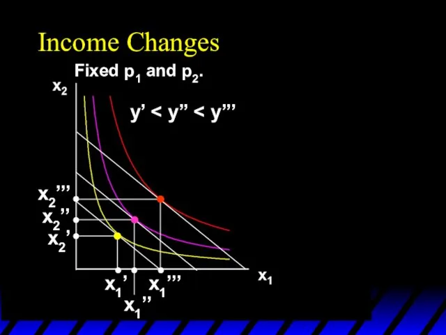
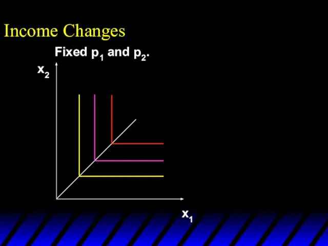
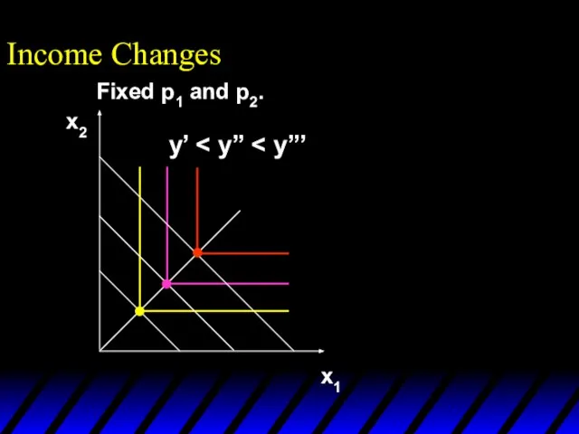
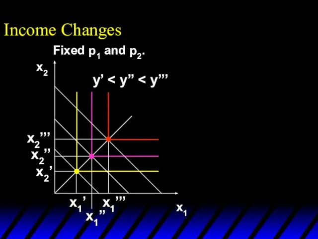
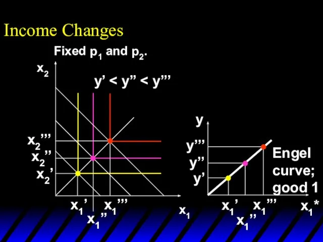
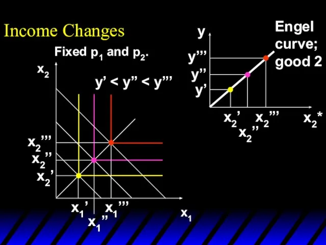
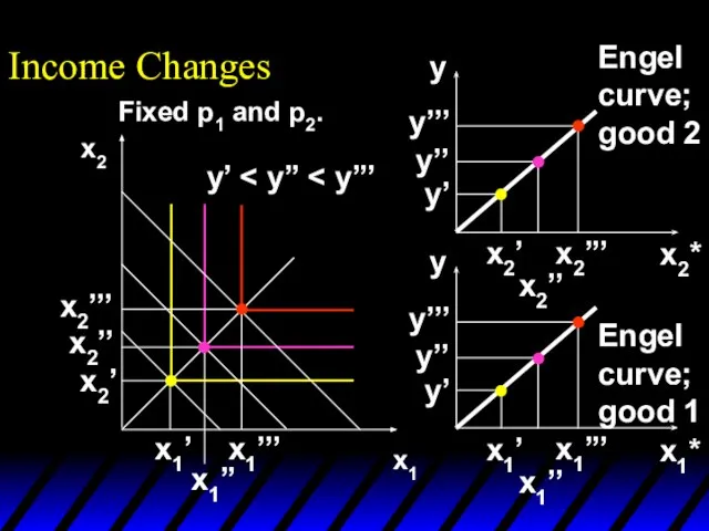
- 59. Income Changes How does the value of x1*(p1,p2,y) change as y changes, holding both p1 and
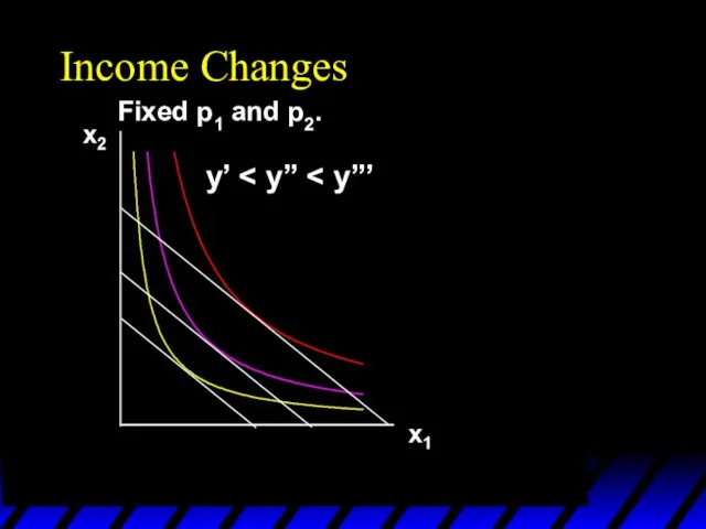
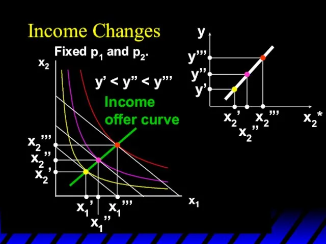
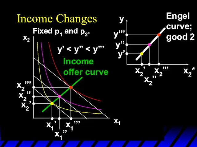
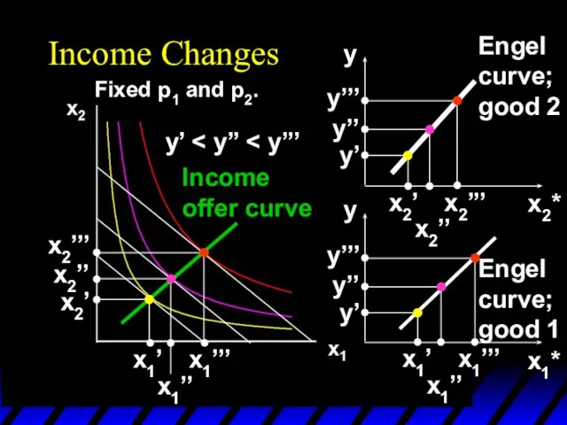
- 60. Income Changes Fixed p1 and p2. y’
- 61. Income Changes Fixed p1 and p2. y’
- 62. Income Changes Fixed p1 and p2. y’ x1’’’ x1’’ x1’ x2’’’ x2’’ x2’
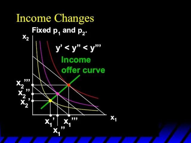
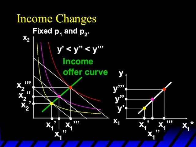
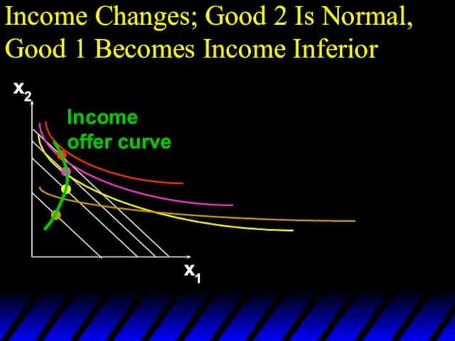
- 63. Income Changes Fixed p1 and p2. y’ x1’’’ x1’’ x1’ x2’’’ x2’’ x2’ Income offer curve
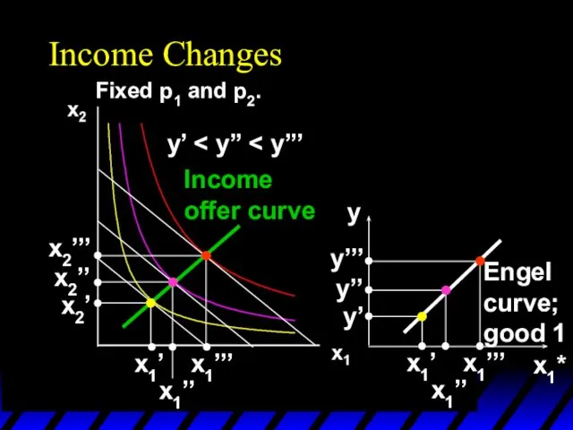
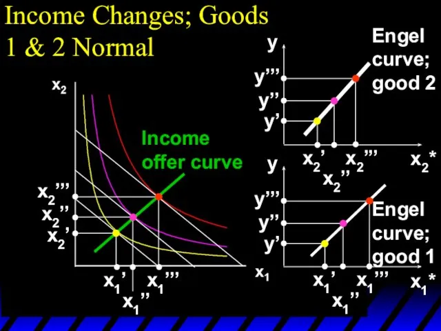
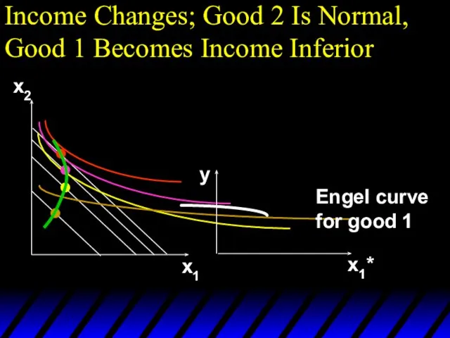
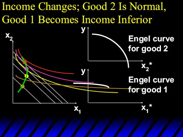
- 64. Income Changes A plot of quantity demanded against income is called an Engel curve.
- 65. Income Changes Fixed p1 and p2. y’ x1’’’ x1’’ x1’ x2’’’ x2’’ x2’ Income offer curve
- 66. Income Changes Fixed p1 and p2. y’ x1’’’ x1’’ x1’ x2’’’ x2’’ x2’ Income offer curve
- 67. Income Changes Fixed p1 and p2. y’ x1’’’ x1’’ x1’ x2’’’ x2’’ x2’ Income offer curve
- 68. Income Changes Fixed p1 and p2. y’ x1’’’ x1’’ x1’ x2’’’ x2’’ x2’ Income offer curve
- 69. Income Changes Fixed p1 and p2. y’ x1’’’ x1’’ x1’ x2’’’ x2’’ x2’ Income offer curve
- 70. Income Changes Fixed p1 and p2. y’ x1’’’ x1’’ x1’ x2’’’ x2’’ x2’ Income offer curve
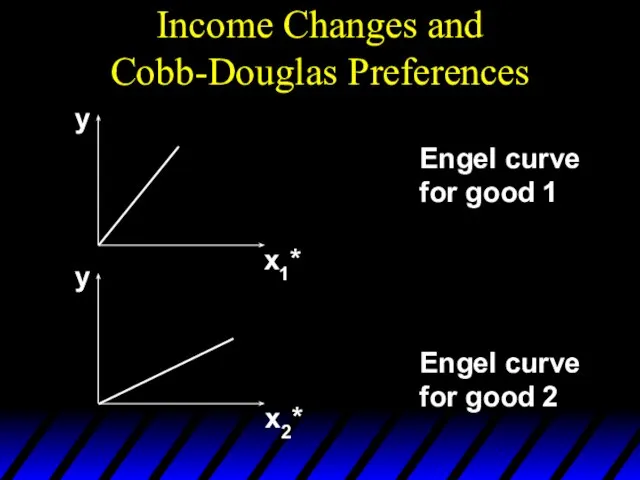
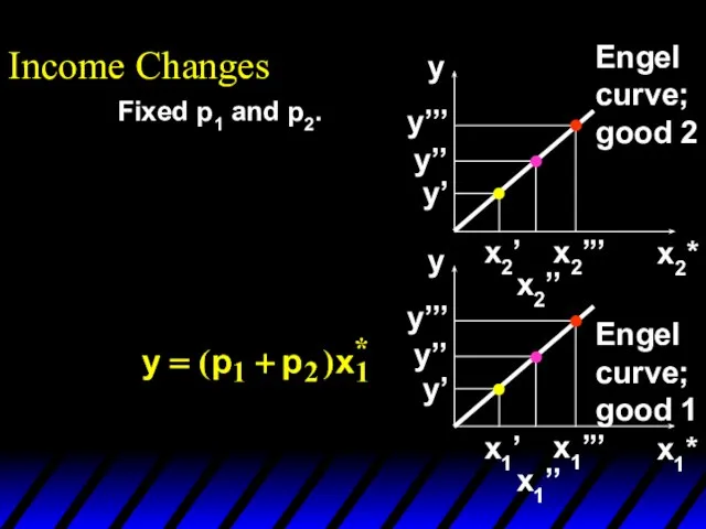
- 71. Income Changes and Cobb-Douglas Preferences An example of computing the equations of Engel curves; the Cobb-Douglas
- 72. Income Changes and Cobb-Douglas Preferences Rearranged to isolate y, these are: Engel curve for good 1
- 73. Income Changes and Cobb-Douglas Preferences y y x1* x2* Engel curve for good 1 Engel curve
- 74. Income Changes and Perfectly-Complementary Preferences Another example of computing the equations of Engel curves; the perfectly-complementary
- 75. Income Changes and Perfectly-Complementary Preferences Rearranged to isolate y, these are: Engel curve for good 1
- 76. Fixed p1 and p2. Income Changes x1 x2
- 77. Income Changes x1 x2 y’ Fixed p1 and p2.
- 78. Income Changes x1 x2 y’ Fixed p1 and p2.
- 79. Income Changes x1 x2 y’ x1’’ x1’ x2’’’ x2’’ x2’ x1’’’ Fixed p1 and p2.
- 80. Income Changes x1 x2 y’ x1’’ x1’ x2’’’ x2’’ x2’ x1’’’ x1* y y’ y’’ y’’’
- 81. Income Changes x1 x2 y’ x1’’ x1’ x2’’’ x2’’ x2’ x1’’’ x2* y x2’’’ x2’’ x2’
- 82. Income Changes x1 x2 y’ x1’’ x1’ x2’’’ x2’’ x2’ x1’’’ x1* x2* y y x2’’’
- 83. Income Changes x1* x2* y y x2’’’ x2’’ x2’ y’ y’’ y’’’ y’ y’’ y’’’ x1’’’
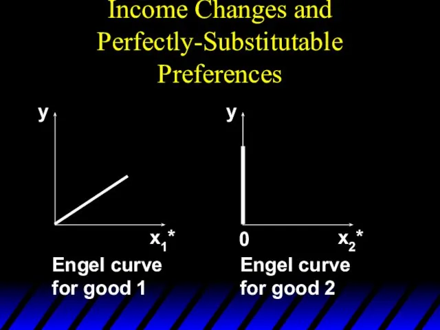
- 84. Income Changes and Perfectly-Substitutable Preferences Another example of computing the equations of Engel curves; the perfectly-substitution
- 85. Income Changes and Perfectly-Substitutable Preferences
- 86. Income Changes and Perfectly-Substitutable Preferences Suppose p1
- 87. Income Changes and Perfectly-Substitutable Preferences Suppose p1 and
- 88. Income Changes and Perfectly-Substitutable Preferences Suppose p1 and and
- 89. Income Changes and Perfectly-Substitutable Preferences y y x1* x2* 0 Engel curve for good 1 Engel
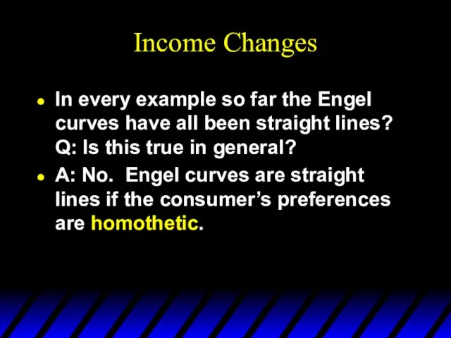
- 90. Income Changes In every example so far the Engel curves have all been straight lines? Q:
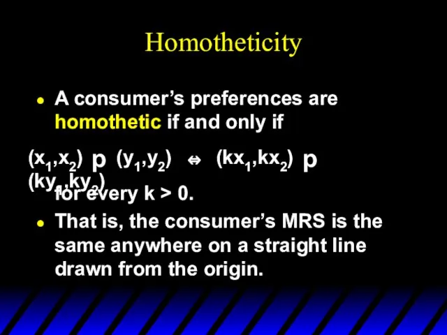
- 91. Homotheticity A consumer’s preferences are homothetic if and only if for every k > 0. That
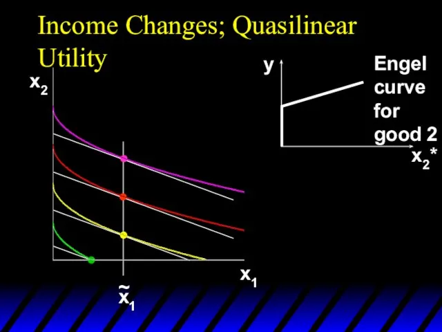
- 92. Income Effects -- A Nonhomothetic Example Quasilinear preferences are not homothetic. For example,
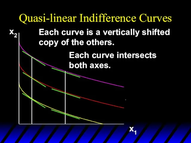
- 93. Quasi-linear Indifference Curves x2 x1 Each curve is a vertically shifted copy of the others. Each
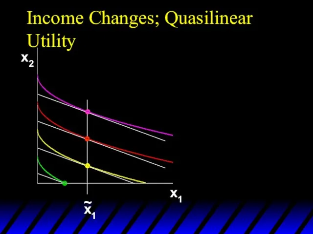
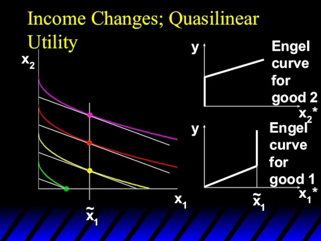
- 94. Income Changes; Quasilinear Utility x2 x1
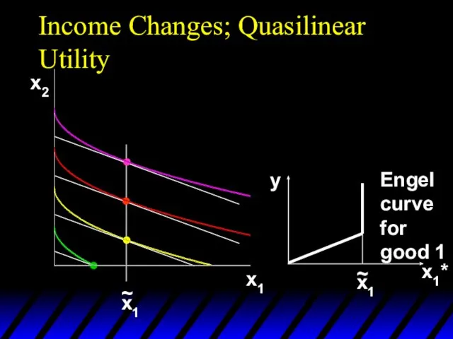
- 95. Income Changes; Quasilinear Utility x2 x1 x1* y x1 ~ Engel curve for good 1
- 96. Income Changes; Quasilinear Utility x2 x1 x2* y Engel curve for good 2
- 97. Income Changes; Quasilinear Utility x2 x1 x1* x2* y y x1 ~ Engel curve for good
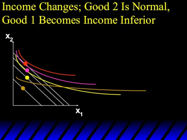
- 98. Income Effects A good for which quantity demanded rises with income is called normal. Therefore a
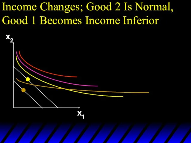
- 99. Income Effects A good for which quantity demanded falls as income increases is called income inferior.
- 100. Income Effects In the US over last hundred years income increased many times whereas the number
- 101. Income Changes; Goods 1 & 2 Normal x1’’’ x1’’ x1’ x2’’’ x2’’ x2’ Income offer curve
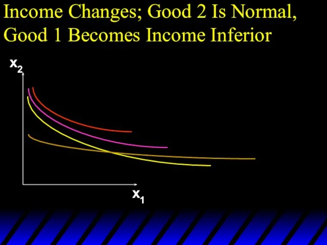
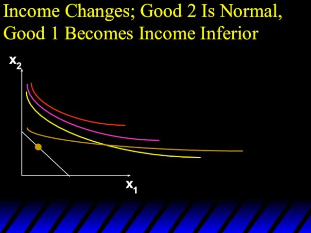
- 102. Income Changes; Good 2 Is Normal, Good 1 Becomes Income Inferior x2 x1
- 103. Income Changes; Good 2 Is Normal, Good 1 Becomes Income Inferior x2 x1
- 104. Income Changes; Good 2 Is Normal, Good 1 Becomes Income Inferior x2 x1
- 105. Income Changes; Good 2 Is Normal, Good 1 Becomes Income Inferior x2 x1
- 106. Income Changes; Good 2 Is Normal, Good 1 Becomes Income Inferior x2 x1
- 107. Income Changes; Good 2 Is Normal, Good 1 Becomes Income Inferior x2 x1 Income offer curve
- 108. Income Changes; Good 2 Is Normal, Good 1 Becomes Income Inferior x2 x1 x1* y Engel
- 109. Income Changes; Good 2 Is Normal, Good 1 Becomes Income Inferior x2 x1 x1* x2* y
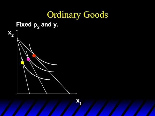
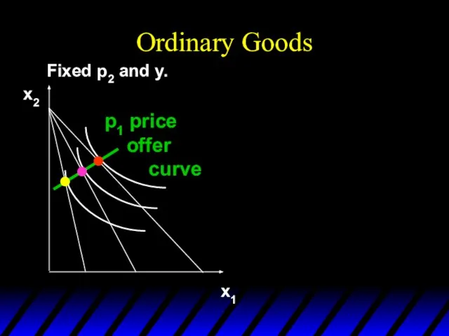
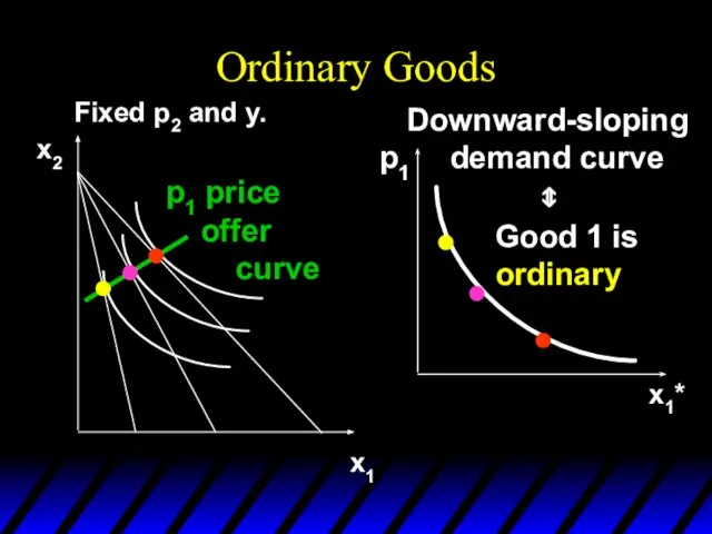
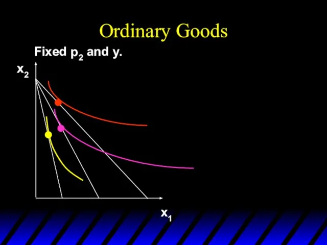
- 110. Ordinary Goods A good is called ordinary if the quantity demanded of it always increases as
- 111. Ordinary Goods Fixed p2 and y. x1 x2
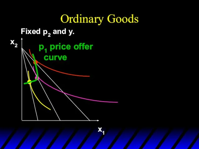
- 112. Ordinary Goods Fixed p2 and y. x1 x2 p1 price offer curve
- 113. Ordinary Goods Fixed p2 and y. x1 x2 p1 price offer curve x1* Downward-sloping demand curve
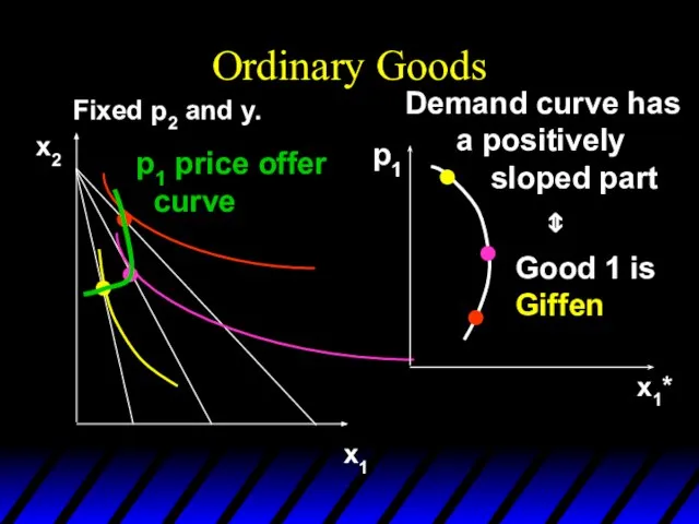
- 114. Giffen Goods If, for some values of its own price, the quantity demanded of a good
- 115. Ordinary Goods Fixed p2 and y. x1 x2
- 116. Ordinary Goods Fixed p2 and y. x1 x2 p1 price offer curve
- 117. Ordinary Goods Fixed p2 and y. x1 x2 p1 price offer curve x1* Demand curve has
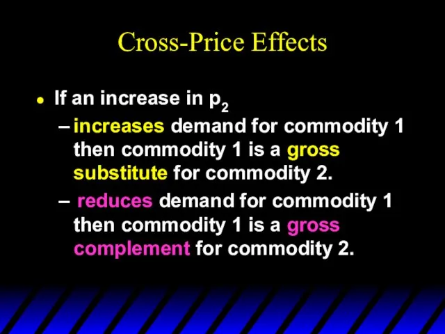
- 118. Cross-Price Effects If an increase in p2 increases demand for commodity 1 then commodity 1 is
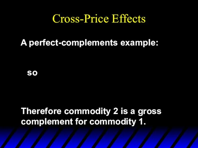
- 119. Cross-Price Effects A perfect-complements example: so Therefore commodity 2 is a gross complement for commodity 1.
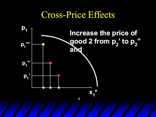
- 120. Cross-Price Effects p1 x1* p1’ p1’’ p1’’’ Increase the price of good 2 from p2’ to
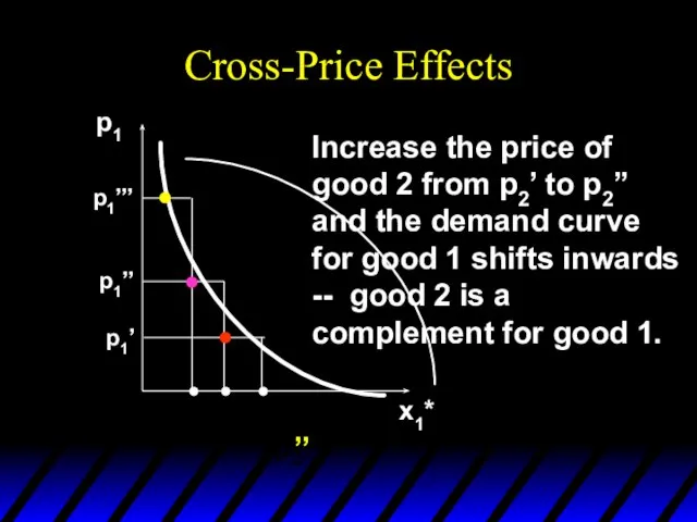
- 121. Cross-Price Effects p1 x1* p1’ p1’’ p1’’’ Increase the price of good 2 from p2’ to
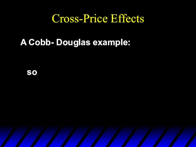
- 122. Cross-Price Effects A Cobb- Douglas example: so
- 124. Скачать презентацию
Слайд 2Properties of Demand Functions
Comparative statics analysis of ordinary demand functions -- the
Properties of Demand Functions
Comparative statics analysis of ordinary demand functions -- the
Слайд 3Own-Price Changes
How does x1*(p1,p2,y) change as p1 changes, holding p2 and y
Own-Price Changes
How does x1*(p1,p2,y) change as p1 changes, holding p2 and y
Слайд 4
x1
x2
p1 = p1’
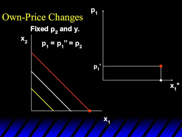
Fixed p2 and y.
p1x1 + p2x2 = y
Own-Price Changes
x1
x2
p1 = p1’
Fixed p2 and y.
p1x1 + p2x2 = y
Own-Price Changes
Слайд 5Own-Price Changes
x1
x2
p1= p1’’
p1 = p1’
Fixed p2 and y.
p1x1 + p2x2 = y
Own-Price Changes
x1
x2
p1= p1’’
p1 = p1’
Fixed p2 and y.
p1x1 + p2x2 = y
Слайд 6Own-Price Changes
x1
x2
p1= p1’’
p1=
p1’’’
Fixed p2 and y.
p1 = p1’
p1x1 + p2x2 = y
Own-Price Changes
x1
x2
p1= p1’’
p1=
p1’’’
Fixed p2 and y.
p1 = p1’
p1x1 + p2x2 = y
Слайд 7p1 = p1’
Own-Price Changes
Fixed p2 and y.
p1 = p1’
Own-Price Changes
Fixed p2 and y.
Слайд 8x1*(p1’)
Own-Price Changes
p1 = p1’
Fixed p2 and y.
x1*(p1’)
Own-Price Changes
p1 = p1’
Fixed p2 and y.
Слайд 9x1*(p1’)
p1
x1*(p1’)
p1’
x1*
Own-Price Changes
Fixed p2 and y.
p1 = p1’
x1*(p1’)
p1
x1*(p1’)
p1’
x1*
Own-Price Changes
Fixed p2 and y.
p1 = p1’
Слайд 10x1*(p1’)
p1
x1*(p1’)
p1’
p1 = p1’’
x1*
Own-Price Changes
Fixed p2 and y.
x1*(p1’)
p1
x1*(p1’)
p1’
p1 = p1’’
x1*
Own-Price Changes
Fixed p2 and y.
Слайд 11x1*(p1’)
x1*(p1’’)
p1
x1*(p1’)
p1’
p1 = p1’’
x1*
Own-Price Changes
Fixed p2 and y.
x1*(p1’)
x1*(p1’’)
p1
x1*(p1’)
p1’
p1 = p1’’
x1*
Own-Price Changes
Fixed p2 and y.
Слайд 12x1*(p1’)
x1*(p1’’)
p1
x1*(p1’)
x1*(p1’’)
p1’
p1’’
x1*
Own-Price Changes
Fixed p2 and y.
x1*(p1’)
x1*(p1’’)
p1
x1*(p1’)
x1*(p1’’)
p1’
p1’’
x1*
Own-Price Changes
Fixed p2 and y.
Слайд 13x1*(p1’)
x1*(p1’’)
p1
x1*(p1’)
x1*(p1’’)
p1’
p1’’
p1 = p1’’’
x1*
Own-Price Changes
Fixed p2 and y.
x1*(p1’)
x1*(p1’’)
p1
x1*(p1’)
x1*(p1’’)
p1’
p1’’
p1 = p1’’’
x1*
Own-Price Changes
Fixed p2 and y.
Слайд 14x1*(p1’’’)
x1*(p1’)
x1*(p1’’)
p1
x1*(p1’)
x1*(p1’’)
p1’
p1’’
p1 = p1’’’
x1*
Own-Price Changes
Fixed p2 and y.
x1*(p1’’’)
x1*(p1’)
x1*(p1’’)
p1
x1*(p1’)
x1*(p1’’)
p1’
p1’’
p1 = p1’’’
x1*
Own-Price Changes
Fixed p2 and y.
Слайд 15x1*(p1’’’)
x1*(p1’)
x1*(p1’’)
p1
x1*(p1’)
x1*(p1’’’)
x1*(p1’’)
p1’
p1’’
p1’’’
x1*
Own-Price Changes
Fixed p2 and y.
x1*(p1’’’)
x1*(p1’)
x1*(p1’’)
p1
x1*(p1’)
x1*(p1’’’)
x1*(p1’’)
p1’
p1’’
p1’’’
x1*
Own-Price Changes
Fixed p2 and y.
Слайд 16x1*(p1’’’)
x1*(p1’)
x1*(p1’’)
p1
x1*(p1’)
x1*(p1’’’)
x1*(p1’’)
p1’
p1’’
p1’’’
x1*
Own-Price Changes
Ordinary
demand curve
for commodity 1
Fixed p2 and y.
x1*(p1’’’)
x1*(p1’)
x1*(p1’’)
p1
x1*(p1’)
x1*(p1’’’)
x1*(p1’’)
p1’
p1’’
p1’’’
x1*
Own-Price Changes
Ordinary
demand curve
for commodity 1
Fixed p2 and y.
Слайд 17x1*(p1’’’)
x1*(p1’)
x1*(p1’’)
p1
x1*(p1’)
x1*(p1’’’)
x1*(p1’’)
p1’
p1’’
p1’’’
x1*
Own-Price Changes
Ordinary
demand curve
for commodity 1
Fixed p2 and y.
x1*(p1’’’)
x1*(p1’)
x1*(p1’’)
p1
x1*(p1’)
x1*(p1’’’)
x1*(p1’’)
p1’
p1’’
p1’’’
x1*
Own-Price Changes
Ordinary
demand curve
for commodity 1
Fixed p2 and y.
Слайд 18x1*(p1’’’)
x1*(p1’)
x1*(p1’’)
p1
x1*(p1’)
x1*(p1’’’)
x1*(p1’’)
p1’
p1’’
p1’’’
x1*
Own-Price Changes
Ordinary
demand curve
for commodity 1
p1 price
offer
curve
Fixed p2 and y.
x1*(p1’’’)
x1*(p1’)
x1*(p1’’)
p1
x1*(p1’)
x1*(p1’’’)
x1*(p1’’)
p1’
p1’’
p1’’’
x1*
Own-Price Changes
Ordinary
demand curve
for commodity 1
p1 price
offer
curve
Fixed p2 and y.
Слайд 19Own-Price Changes
The curve containing all the utility-maximizing bundles traced out as p1
Own-Price Changes
The curve containing all the utility-maximizing bundles traced out as p1
Слайд 20Own-Price Changes
What does a p1 price-offer curve look like for Cobb-Douglas preferences?
Own-Price Changes
What does a p1 price-offer curve look like for Cobb-Douglas preferences?

Слайд 21Own-Price Changes
What does a p1 price-offer curve look like for Cobb-Douglas preferences?
Take
Then
Own-Price Changes
What does a p1 price-offer curve look like for Cobb-Douglas preferences?
Take
Then
Слайд 22Own-Price Changes
and
Notice that x2* does not vary with p1 so the
p1 price
Own-Price Changes
and
Notice that x2* does not vary with p1 so the p1 price
Слайд 23Own-Price Changes
and
Notice that x2* does not vary with p1 so the
p1 price
Own-Price Changes
and
Notice that x2* does not vary with p1 so the p1 price
Слайд 24Own-Price Changes
and
Notice that x2* does not vary with p1 so the
p1 price
Own-Price Changes
and
Notice that x2* does not vary with p1 so the p1 price
Слайд 25Own-Price Changes
and
Notice that x2* does not vary with p1 so the
p1 price
Own-Price Changes
and
Notice that x2* does not vary with p1 so the p1 price
Слайд 26x1*(p1’’’)
x1*(p1’)
x1*(p1’’)
Own-Price Changes
Fixed p2 and y.
x1*(p1’’’)
x1*(p1’)
x1*(p1’’)
Own-Price Changes
Fixed p2 and y.
Слайд 27x1*(p1’’’)
x1*(p1’)
x1*(p1’’)
p1
x1*
Own-Price Changes
Ordinary
demand curve
for commodity 1
is
Fixed p2 and y.
x1*(p1’’’)
x1*(p1’)
x1*(p1’’)
p1
x1*
Own-Price Changes
Ordinary
demand curve
for commodity 1
is
Fixed p2 and y.
Слайд 28Own-Price Changes
What does a p1 price-offer curve look like for a perfect-complements
Own-Price Changes
What does a p1 price-offer curve look like for a perfect-complements

Слайд 29Own-Price Changes
What does a p1 price-offer curve look like for a perfect-complements
Own-Price Changes
What does a p1 price-offer curve look like for a perfect-complements
Слайд 30Own-Price Changes
Own-Price Changes

Слайд 31Own-Price Changes
With p2 and y fixed, higher p1 causes
smaller x1* and x2*.
Own-Price Changes
With p2 and y fixed, higher p1 causes
smaller x1* and x2*.
Слайд 32Own-Price Changes
With p2 and y fixed, higher p1 causes
smaller x1* and x2*.
As
Own-Price Changes
With p2 and y fixed, higher p1 causes
smaller x1* and x2*.
As
Слайд 33Own-Price Changes
With p2 and y fixed, higher p1 causes
smaller x1* and x2*.
As
As
Own-Price Changes
With p2 and y fixed, higher p1 causes
smaller x1* and x2*.
As
As
Слайд 34Fixed p2 and y.
Own-Price Changes
x1
x2
Fixed p2 and y.
Own-Price Changes
x1
x2
Слайд 35p1
x1*
Fixed p2 and y.
Own-Price Changes
x1
x2
p1’
’
p1 = p1’
’
’
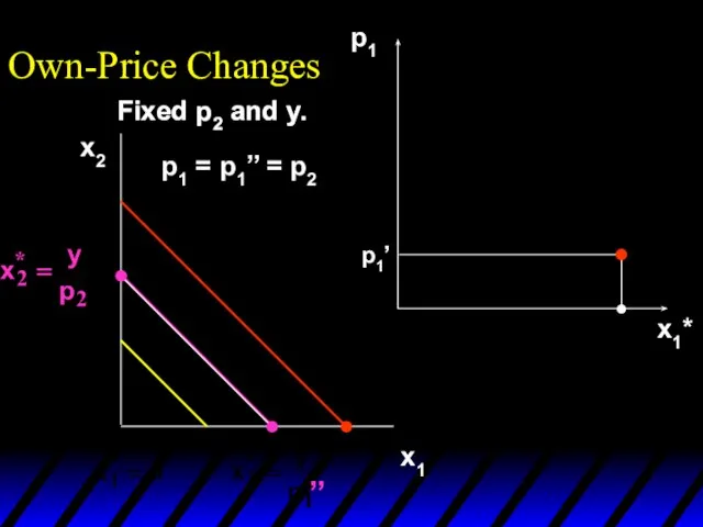
y/p2
p1
x1*
Fixed p2 and y.
Own-Price Changes
x1
x2
p1’
’
p1 = p1’
’
’
y/p2
Слайд 36p1
x1*
Fixed p2 and y.
Own-Price Changes
x1
x2
p1’
p1’’
p1 = p1’’
’’
’’
’’
y/p2
p1
x1*
Fixed p2 and y.
Own-Price Changes
x1
x2
p1’
p1’’
p1 = p1’’
’’
’’
’’
y/p2
Слайд 37p1
x1*
Fixed p2 and y.
Own-Price Changes
x1
x2
p1’
p1’’
p1’’’
p1 = p1’’’
’’’
’’’
’’’
y/p2
p1
x1*
Fixed p2 and y.
Own-Price Changes
x1
x2
p1’
p1’’
p1’’’
p1 = p1’’’
’’’
’’’
’’’
y/p2
Слайд 38p1
x1*
Ordinary
demand curve
for commodity 1
is
Fixed p2 and y.
Own-Price Changes
x1
x2
p1’
p1’’
p1’’’
y/p2
p1
x1*
Ordinary
demand curve
for commodity 1
is
Fixed p2 and y.
Own-Price Changes
x1
x2
p1’
p1’’
p1’’’
y/p2
Слайд 39Own-Price Changes
What does a p1 price-offer curve look like for a perfect-substitutes
Own-Price Changes
What does a p1 price-offer curve look like for a perfect-substitutes
Слайд 40Own-Price Changes
and
Own-Price Changes
and

Слайд 41Fixed p2 and y.
Own-Price Changes
x2
x1
Fixed p2 and y.
p1 = p1’ < p2
’
Fixed p2 and y.
Own-Price Changes
x2
x1
Fixed p2 and y.
p1 = p1’ < p2
’
Слайд 42Fixed p2 and y.
Own-Price Changes
x2
x1
p1
x1*
Fixed p2 and y.
p1’
p1 = p1’ < p2
’
’
Fixed p2 and y.
Own-Price Changes
x2
x1
p1
x1*
Fixed p2 and y.
p1’
p1 = p1’ < p2
’
’
Слайд 43Fixed p2 and y.
Own-Price Changes
x2
x1
p1
x1*
Fixed p2 and y.
p1’
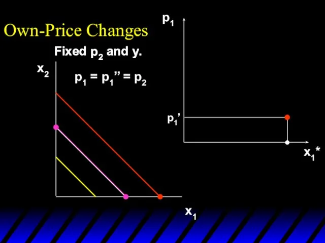
p1 = p1’’ = p2
Fixed p2 and y.
Own-Price Changes
x2
x1
p1
x1*
Fixed p2 and y.
p1’
p1 = p1’’ = p2
Слайд 44Fixed p2 and y.
Own-Price Changes
x2
x1
p1
x1*
Fixed p2 and y.
p1’
p1 = p1’’ = p2
Fixed p2 and y.
Own-Price Changes
x2
x1
p1
x1*
Fixed p2 and y.
p1’
p1 = p1’’ = p2
Слайд 45Fixed p2 and y.
Own-Price Changes
x2
x1
p1
x1*
Fixed p2 and y.
p1’
p1 = p1’’ = p2
’’
Fixed p2 and y.
Own-Price Changes
x2
x1
p1
x1*
Fixed p2 and y.
p1’
p1 = p1’’ = p2
’’
Слайд 46Fixed p2 and y.
Own-Price Changes
x2
x1
p1
x1*
Fixed p2 and y.
p1’
p1 = p1’’ = p2
p2
Fixed p2 and y.
Own-Price Changes
x2
x1
p1
x1*
Fixed p2 and y.
p1’
p1 = p1’’ = p2
p2
Слайд 47Fixed p2 and y.
Own-Price Changes
x2
x1
p1
x1*
Fixed p2 and y.
p1’
p1’’’
p2 = p1’’
Fixed p2 and y.
Own-Price Changes
x2
x1
p1
x1*
Fixed p2 and y.
p1’
p1’’’
p2 = p1’’
Слайд 48Fixed p2 and y.
Own-Price Changes
x2
x1
p1
x1*
Fixed p2 and y.
p1’
p2 = p1’’
p1’’’
p1 price
offer
Fixed p2 and y.
Own-Price Changes
x2
x1
p1
x1*
Fixed p2 and y.
p1’
p2 = p1’’
p1’’’
p1 price
offer
Слайд 49Own-Price Changes
Usually we ask “Given the price for commodity 1 what is
Own-Price Changes
Usually we ask “Given the price for commodity 1 what is
Слайд 50Own-Price Changes
p1
x1*
p1’
Given p1’, what quantity is
demanded of commodity 1?
Own-Price Changes
p1
x1*
p1’
Given p1’, what quantity is
demanded of commodity 1?
Слайд 51Own-Price Changes
p1
x1*
p1’
Given p1’, what quantity is
demanded of commodity 1?
Answer: x1’ units.
x1’
Own-Price Changes
p1
x1*
p1’
Given p1’, what quantity is
demanded of commodity 1?
Answer: x1’ units.
x1’
Слайд 52Own-Price Changes
p1
x1*
x1’
Given p1’, what quantity is
demanded of commodity 1?
Answer: x1’ units.
The inverse
Own-Price Changes
p1
x1*
x1’
Given p1’, what quantity is
demanded of commodity 1?
Answer: x1’ units.
The inverse
Слайд 53Own-Price Changes
p1
x1*
p1’
x1’
Given p1’, what quantity is
demanded of commodity 1?
Answer: x1’ units.
The inverse
Own-Price Changes
p1
x1*
p1’
x1’
Given p1’, what quantity is
demanded of commodity 1?
Answer: x1’ units.
The inverse
Слайд 54Own-Price Changes
Taking quantity demanded as given and then asking what must be
Own-Price Changes
Taking quantity demanded as given and then asking what must be
Слайд 55Own-Price Changes
Inverse demand function
At optimal choice
|MRS| = p1/p2
Therefore:
p1 = p2 |MRS|
Own-Price Changes
Inverse demand function
At optimal choice
|MRS| = p1/p2
Therefore:
p1 = p2 |MRS|
Слайд 56Own-Price Changes
Inverse demand function
If good 2 is money, then MRS (and inverse
Own-Price Changes
Inverse demand function
If good 2 is money, then MRS (and inverse
Слайд 57Own-Price Changes
A Cobb-Douglas example:
is the ordinary demand function and
is the inverse demand
Own-Price Changes
A Cobb-Douglas example:
is the ordinary demand function and
is the inverse demand
Слайд 58Own-Price Changes
A perfect-complements example:
is the ordinary demand function and
is the inverse demand
Own-Price Changes
A perfect-complements example:
is the ordinary demand function and
is the inverse demand
Слайд 59Income Changes
How does the value of x1*(p1,p2,y) change as y changes, holding
Income Changes
How does the value of x1*(p1,p2,y) change as y changes, holding
Слайд 60Income Changes
Fixed p1 and p2.
y’ < y’’ < y’’’
Income Changes
Fixed p1 and p2.
y’ < y’’ < y’’’
Слайд 61Income Changes
Fixed p1 and p2.
y’ < y’’ < y’’’
Income Changes
Fixed p1 and p2.
y’ < y’’ < y’’’
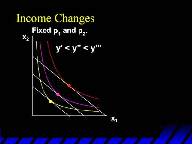
Слайд 62Income Changes
Fixed p1 and p2.
y’ < y’’ < y’’’
x1’’’
x1’’
x1’
x2’’’
x2’’
x2’
Income Changes
Fixed p1 and p2.
y’ < y’’ < y’’’
x1’’’
x1’’
x1’
x2’’’
x2’’
x2’
Слайд 63Income Changes
Fixed p1 and p2.
y’ < y’’ < y’’’
x1’’’
x1’’
x1’
x2’’’
x2’’
x2’
Income
offer curve
Income Changes
Fixed p1 and p2.
y’ < y’’ < y’’’
x1’’’
x1’’
x1’
x2’’’
x2’’
x2’
Income
offer curve

Слайд 64Income Changes
A plot of quantity demanded against income is called an Engel
Income Changes
A plot of quantity demanded against income is called an Engel

Слайд 65Income Changes
Fixed p1 and p2.
y’ < y’’ < y’’’
x1’’’
x1’’
x1’
x2’’’
x2’’
x2’
Income
offer curve
Income Changes
Fixed p1 and p2.
y’ < y’’ < y’’’
x1’’’
x1’’
x1’
x2’’’
x2’’
x2’
Income
offer curve
Слайд 66Income Changes
Fixed p1 and p2.
y’ < y’’ < y’’’
x1’’’
x1’’
x1’
x2’’’
x2’’
x2’
Income
offer curve
x1*
y
x1’’’
x1’’
x1’
y’
y’’
y’’’
Income Changes
Fixed p1 and p2.
y’ < y’’ < y’’’
x1’’’
x1’’
x1’
x2’’’
x2’’
x2’
Income
offer curve
x1*
y
x1’’’
x1’’
x1’
y’
y’’
y’’’
Слайд 67Income Changes
Fixed p1 and p2.
y’ < y’’ < y’’’
x1’’’
x1’’
x1’
x2’’’
x2’’
x2’
Income
offer curve
x1*
y
x1’’’
x1’’
x1’
y’
y’’
y’’’
Engel
curve;
good 1
Income Changes
Fixed p1 and p2.
y’ < y’’ < y’’’
x1’’’
x1’’
x1’
x2’’’
x2’’
x2’
Income
offer curve
x1*
y
x1’’’
x1’’
x1’
y’
y’’
y’’’
Engel
curve;
good 1
Слайд 68Income Changes
Fixed p1 and p2.
y’ < y’’ < y’’’
x1’’’
x1’’
x1’
x2’’’
x2’’
x2’
Income
offer curve
x2*
y
x2’’’
x2’’
x2’
y’
y’’
y’’’
Income Changes
Fixed p1 and p2.
y’ < y’’ < y’’’
x1’’’
x1’’
x1’
x2’’’
x2’’
x2’
Income
offer curve
x2*
y
x2’’’
x2’’
x2’
y’
y’’
y’’’
Слайд 69Income Changes
Fixed p1 and p2.
y’ < y’’ < y’’’
x1’’’
x1’’
x1’
x2’’’
x2’’
x2’
Income
offer curve
x2*
y
x2’’’
x2’’
x2’
y’
y’’
y’’’
Engel
curve;
good 2
Income Changes
Fixed p1 and p2.
y’ < y’’ < y’’’
x1’’’
x1’’
x1’
x2’’’
x2’’
x2’
Income
offer curve
x2*
y
x2’’’
x2’’
x2’
y’
y’’
y’’’
Engel
curve;
good 2
Слайд 70Income Changes
Fixed p1 and p2.
y’ < y’’ < y’’’
x1’’’
x1’’
x1’
x2’’’
x2’’
x2’
Income
offer curve
x1*
x2*
y
y
x1’’’
x1’’
x1’
x2’’’
x2’’
x2’
y’
y’’
y’’’
y’
y’’
y’’’
Engel
curve;
good 2
Engel
curve;
good 1
Income Changes
Fixed p1 and p2.
y’ < y’’ < y’’’
x1’’’
x1’’
x1’
x2’’’
x2’’
x2’
Income
offer curve
x1*
x2*
y
y
x1’’’
x1’’
x1’
x2’’’
x2’’
x2’
y’
y’’
y’’’
y’
y’’
y’’’
Engel
curve;
good 2
Engel
curve;
good 1
Слайд 71Income Changes and Cobb-Douglas Preferences
An example of computing the equations of Engel
Income Changes and Cobb-Douglas Preferences
An example of computing the equations of Engel
Слайд 72Income Changes and Cobb-Douglas Preferences
Rearranged to isolate y, these are:
Engel curve for
Income Changes and Cobb-Douglas Preferences
Rearranged to isolate y, these are:
Engel curve for

Слайд 73Income Changes and Cobb-Douglas Preferences
y
y
x1*
x2*
Engel curve
for good 1
Engel curve
for good 2
Income Changes and Cobb-Douglas Preferences
y
y
x1*
x2*
Engel curve
for good 1
Engel curve
for good 2
Слайд 74Income Changes and Perfectly-Complementary Preferences
Another example of computing the equations of Engel
Income Changes and Perfectly-Complementary Preferences
Another example of computing the equations of Engel

Слайд 75Income Changes and Perfectly-Complementary Preferences
Rearranged to isolate y, these are:
Engel curve for
Income Changes and Perfectly-Complementary Preferences
Rearranged to isolate y, these are:
Engel curve for

Слайд 76Fixed p1 and p2.
Income Changes
x1
x2
Fixed p1 and p2.
Income Changes
x1
x2
Слайд 77Income Changes
x1
x2
y’ < y’’ < y’’’
Fixed p1 and p2.
Income Changes
x1
x2
y’ < y’’ < y’’’
Fixed p1 and p2.

Слайд 78Income Changes
x1
x2
y’ < y’’ < y’’’
Fixed p1 and p2.
Income Changes
x1
x2
y’ < y’’ < y’’’
Fixed p1 and p2.
Слайд 79Income Changes
x1
x2
y’ < y’’ < y’’’
x1’’
x1’
x2’’’
x2’’
x2’
x1’’’
Fixed p1 and p2.
Income Changes
x1
x2
y’ < y’’ < y’’’
x1’’
x1’
x2’’’
x2’’
x2’
x1’’’
Fixed p1 and p2.
Слайд 80Income Changes
x1
x2
y’ < y’’ < y’’’
x1’’
x1’
x2’’’
x2’’
x2’
x1’’’
x1*
y
y’
y’’
y’’’
Engel
curve;
good 1
x1’’’
x1’’
x1’
Fixed p1 and p2.
Income Changes
x1
x2
y’ < y’’ < y’’’
x1’’
x1’
x2’’’
x2’’
x2’
x1’’’
x1*
y
y’
y’’
y’’’
Engel
curve;
good 1
x1’’’
x1’’
x1’
Fixed p1 and p2.
Слайд 81Income Changes
x1
x2
y’ < y’’ < y’’’
x1’’
x1’
x2’’’
x2’’
x2’
x1’’’
x2*
y
x2’’’
x2’’
x2’
y’
y’’
y’’’
Engel
curve;
good 2
Fixed p1 and p2.
Income Changes
x1
x2
y’ < y’’ < y’’’
x1’’
x1’
x2’’’
x2’’
x2’
x1’’’
x2*
y
x2’’’
x2’’
x2’
y’
y’’
y’’’
Engel
curve;
good 2
Fixed p1 and p2.
Слайд 82Income Changes
x1
x2
y’ < y’’ < y’’’
x1’’
x1’
x2’’’
x2’’
x2’
x1’’’
x1*
x2*
y
y
x2’’’
x2’’
x2’
y’
y’’
y’’’
y’
y’’
y’’’
Engel
curve;
good 2
Engel
curve;
good 1
x1’’’
x1’’
x1’
Fixed p1 and p2.
Income Changes
x1
x2
y’ < y’’ < y’’’
x1’’
x1’
x2’’’
x2’’
x2’
x1’’’
x1*
x2*
y
y
x2’’’
x2’’
x2’
y’
y’’
y’’’
y’
y’’
y’’’
Engel
curve;
good 2
Engel
curve;
good 1
x1’’’
x1’’
x1’
Fixed p1 and p2.
Слайд 83Income Changes
x1*
x2*
y
y
x2’’’
x2’’
x2’
y’
y’’
y’’’
y’
y’’
y’’’
x1’’’
x1’’
x1’
Engel
curve;
good 2
Engel
curve;
good 1
Fixed p1 and p2.
Income Changes
x1*
x2*
y
y
x2’’’
x2’’
x2’
y’
y’’
y’’’
y’
y’’
y’’’
x1’’’
x1’’
x1’
Engel
curve;
good 2
Engel
curve;
good 1
Fixed p1 and p2.
Слайд 84Income Changes and Perfectly-Substitutable Preferences
Another example of computing the equations of Engel
Income Changes and Perfectly-Substitutable Preferences
Another example of computing the equations of Engel
Слайд 85Income Changes and Perfectly-Substitutable Preferences
Income Changes and Perfectly-Substitutable Preferences

Слайд 86Income Changes and Perfectly-Substitutable Preferences
Suppose p1 < p2. Then
Income Changes and Perfectly-Substitutable Preferences
Suppose p1 < p2. Then

Слайд 87Income Changes and Perfectly-Substitutable Preferences
Suppose p1 < p2. Then
and
Income Changes and Perfectly-Substitutable Preferences
Suppose p1 < p2. Then
and

Слайд 88Income Changes and Perfectly-Substitutable Preferences
Suppose p1 < p2. Then
and
and
Income Changes and Perfectly-Substitutable Preferences
Suppose p1 < p2. Then
and
and

Слайд 89Income Changes and Perfectly-Substitutable Preferences
y
y
x1*
x2*
0
Engel curve
for good 1
Engel curve
for good 2
Income Changes and Perfectly-Substitutable Preferences
y
y
x1*
x2*
0
Engel curve
for good 1
Engel curve
for good 2
Слайд 90Income Changes
In every example so far the Engel curves have all been
Income Changes
In every example so far the Engel curves have all been
Слайд 91Homotheticity
A consumer’s preferences are homothetic if and only if
for every k >
Homotheticity
A consumer’s preferences are homothetic if and only if for every k >
Слайд 92Income Effects -- A Nonhomothetic Example
Quasilinear preferences are not homothetic.
For example,
Income Effects -- A Nonhomothetic Example
Quasilinear preferences are not homothetic.
For example,
Слайд 93Quasi-linear Indifference Curves
x2
x1
Each curve is a vertically shifted copy of the others.
Each
Quasi-linear Indifference Curves
x2
x1
Each curve is a vertically shifted copy of the others.
Each
Слайд 94Income Changes; Quasilinear Utility
x2
x1
Income Changes; Quasilinear Utility
x2
x1
Слайд 95Income Changes; Quasilinear Utility
x2
x1
x1*
y
x1
~
Engel
curve
for
good 1
Income Changes; Quasilinear Utility
x2
x1
x1*
y
x1
~
Engel
curve
for
good 1
Слайд 96Income Changes; Quasilinear Utility
x2
x1
x2*
y
Engel
curve
for
good 2
Income Changes; Quasilinear Utility
x2
x1
x2*
y
Engel
curve
for
good 2
Слайд 97Income Changes; Quasilinear Utility
x2
x1
x1*
x2*
y
y
x1
~
Engel
curve
for
good 2
Engel
curve
for
good 1
Income Changes; Quasilinear Utility
x2
x1
x1*
x2*
y
y
x1
~
Engel
curve
for
good 2
Engel
curve
for
good 1
Слайд 98Income Effects
A good for which quantity demanded rises with income is called
Income Effects
A good for which quantity demanded rises with income is called
Слайд 99Income Effects
A good for which quantity demanded falls as income increases is
Income Effects
A good for which quantity demanded falls as income increases is
Слайд 100Income Effects
In the US over last hundred years income increased many times
Income Effects
In the US over last hundred years income increased many times

Слайд 101Income Changes; Goods
1 & 2 Normal
x1’’’
x1’’
x1’
x2’’’
x2’’
x2’
Income
offer curve
x1*
x2*
y
y
x1’’’
x1’’
x1’
x2’’’
x2’’
x2’
y’
y’’
y’’’
y’
y’’
y’’’
Engel
curve;
good 2
Engel
curve;
good 1
Income Changes; Goods
1 & 2 Normal
x1’’’
x1’’
x1’
x2’’’
x2’’
x2’
Income
offer curve
x1*
x2*
y
y
x1’’’
x1’’
x1’
x2’’’
x2’’
x2’
y’
y’’
y’’’
y’
y’’
y’’’
Engel
curve;
good 2
Engel
curve;
good 1
Слайд 102Income Changes; Good 2 Is Normal, Good 1 Becomes Income Inferior
x2
x1
Income Changes; Good 2 Is Normal, Good 1 Becomes Income Inferior
x2
x1
Слайд 103Income Changes; Good 2 Is Normal, Good 1 Becomes Income Inferior
x2
x1
Income Changes; Good 2 Is Normal, Good 1 Becomes Income Inferior
x2
x1
Слайд 104Income Changes; Good 2 Is Normal, Good 1 Becomes Income Inferior
x2
x1
Income Changes; Good 2 Is Normal, Good 1 Becomes Income Inferior
x2
x1
Слайд 105Income Changes; Good 2 Is Normal, Good 1 Becomes Income Inferior
x2
x1
Income Changes; Good 2 Is Normal, Good 1 Becomes Income Inferior
x2
x1

Слайд 106Income Changes; Good 2 Is Normal, Good 1 Becomes Income Inferior
x2
x1
Income Changes; Good 2 Is Normal, Good 1 Becomes Income Inferior
x2
x1
Слайд 107Income Changes; Good 2 Is Normal, Good 1 Becomes Income Inferior
x2
x1
Income
offer curve
Income Changes; Good 2 Is Normal, Good 1 Becomes Income Inferior
x2
x1
Income
offer curve
Слайд 108Income Changes; Good 2 Is Normal, Good 1 Becomes Income Inferior
x2
x1
x1*
y
Engel curve
for
Income Changes; Good 2 Is Normal, Good 1 Becomes Income Inferior
x2
x1
x1*
y
Engel curve for
Слайд 109Income Changes; Good 2 Is Normal, Good 1 Becomes Income Inferior
x2
x1
x1*
x2*
y
y
Engel curve
for
Income Changes; Good 2 Is Normal, Good 1 Becomes Income Inferior
x2
x1
x1*
x2*
y
y
Engel curve for
Слайд 110Ordinary Goods
A good is called ordinary if the quantity demanded of it
Ordinary Goods
A good is called ordinary if the quantity demanded of it

Слайд 111Ordinary Goods
Fixed p2 and y.
x1
x2
Ordinary Goods
Fixed p2 and y.
x1
x2
Слайд 112Ordinary Goods
Fixed p2 and y.
x1
x2
p1 price
offer
curve
Ordinary Goods
Fixed p2 and y.
x1
x2
p1 price
offer
curve
Слайд 113Ordinary Goods
Fixed p2 and y.
x1
x2
p1 price
offer
curve
x1*
Downward-sloping demand curve
Good 1
Ordinary Goods
Fixed p2 and y.
x1
x2
p1 price
offer
curve
x1*
Downward-sloping demand curve
Good 1
Слайд 114Giffen Goods
If, for some values of its own price, the quantity demanded
Giffen Goods
If, for some values of its own price, the quantity demanded
Слайд 115Ordinary Goods
Fixed p2 and y.
x1
x2
Ordinary Goods
Fixed p2 and y.
x1
x2
Слайд 116Ordinary Goods
Fixed p2 and y.
x1
x2
p1 price offer
curve
Ordinary Goods
Fixed p2 and y.
x1
x2
p1 price offer
curve
Слайд 117Ordinary Goods
Fixed p2 and y.
x1
x2
p1 price offer
curve
x1*
Demand curve has
a positively
Ordinary Goods
Fixed p2 and y.
x1
x2
p1 price offer
curve
x1*
Demand curve has
a positively
Слайд 118Cross-Price Effects
If an increase in p2
increases demand for commodity 1 then commodity
Cross-Price Effects
If an increase in p2
increases demand for commodity 1 then commodity
Слайд 119Cross-Price Effects
A perfect-complements example:
so
Therefore commodity 2 is a gross
complement for commodity 1.
Cross-Price Effects
A perfect-complements example:
so
Therefore commodity 2 is a gross
complement for commodity 1.
Слайд 120Cross-Price Effects
p1
x1*
p1’
p1’’
p1’’’
Increase the price of
good 2 from p2’ to p2’’
and
Cross-Price Effects
p1
x1*
p1’
p1’’
p1’’’
Increase the price of
good 2 from p2’ to p2’’
and
Слайд 121Cross-Price Effects
p1
x1*
p1’
p1’’
p1’’’
Increase the price of
good 2 from p2’ to p2’’
and the demand
Cross-Price Effects
p1
x1*
p1’
p1’’
p1’’’
Increase the price of good 2 from p2’ to p2’’ and the demand
Слайд 122Cross-Price Effects
A Cobb- Douglas example:
so
Cross-Price Effects
A Cobb- Douglas example:
so
 Судебный этикет как составляющая культуры уголовно-процессуальной деятельности. Нормативные основы судебного этикета
 Оружие массового поражения
 Модельный ряд грузовых автомобилей Mercedes-Benz
 Энергетика: вчера, сегодня, завтра
 ГИИС ЭБ. Запрос на аннулирование
 Элементы интернет-маркетинга и их взаимодействие
 1. ОСНОВНЫЕ ПОНЯТИЯ Компьютерный исполнитель – это виртуальный объект, действующий в виртуальной среде обитания. Примеры: –Чертеж
 Beerfest
 Красота осени
 Социально-психологическая служба в школе
 Как принимать управленческие решения
 Денежные переводы в Республике Таджикистан
 Темы в Drupal 6 Что нового, и чем оно грозит
 Память в камне
 Помещение для открытия магазина Белорусская косметика
 Огневая подготовка. Версия 3
 Горный Дагестан
 Методические рекомендации по введению модульной системы и системы зачетных единиц Методические рекомендации по разработке рабо
 Внутренний мир болезни
 Техническое обслуживание и ремонт трансформатора ТДТНГ 40500\115\38,5\6,6 кВ Смоленск – 1
 Кинестетик
 Илья Ефимович Репин –великий русский художник
 Václavské náměstí
 Презентация на тему Иван третий (4 класс)
 11 причин инвестировать в Свердловскую область
 Технология установки врезного замка
 Религия и мораль
 Караевское сельское поселение. Золотые руки мастера по бисероплетению