- InformedSearch

Содержание
- 2. Summary Heuristics and Optimal search strategies heuristics hill-climbing algorithms Best-First search A*: optimal search using heuristics
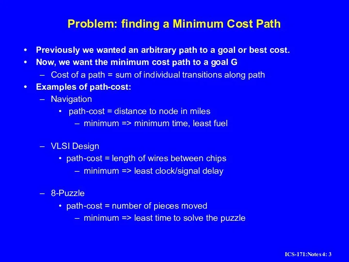
- 3. Problem: finding a Minimum Cost Path Previously we wanted an arbitrary path to a goal or
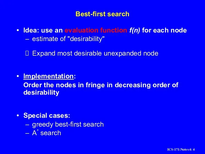
- 4. Best-first search Idea: use an evaluation function f(n) for each node estimate of "desirability" Expand most
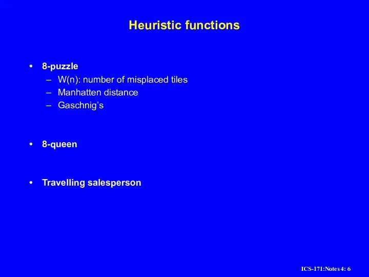
- 5. Heuristic functions 8-puzzle 8-queen Travelling salesperson
- 6. Heuristic functions 8-puzzle W(n): number of misplaced tiles Manhatten distance Gaschnig’s 8-queen Travelling salesperson
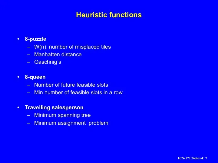
- 7. Heuristic functions 8-puzzle W(n): number of misplaced tiles Manhatten distance Gaschnig’s 8-queen Number of future feasible
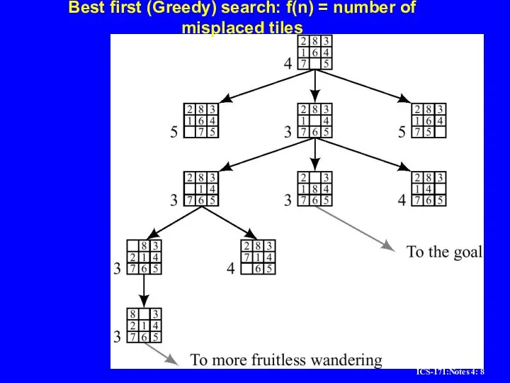
- 8. Best first (Greedy) search: f(n) = number of misplaced tiles
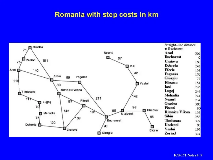
- 9. Romania with step costs in km
- 10. Greedy best-first search Evaluation function f(n) = h(n) (heuristic) = estimate of cost from n to
- 11. Greedy best-first search example
- 12. Greedy best-first search example
- 13. Greedy best-first search example
- 14. Greedy best-first search example
- 15. Problems with Greedy Search Not complete Get stuck on local minimas and plateaus, Irrevocable, Infinite loops
- 16. A* search Idea: avoid expanding paths that are already expensive Evaluation function f(n) = g(n) +
- 17. A* search example
- 18. A* search example
- 19. A* search example
- 20. A* search example
- 21. A* search example
- 22. A* search example
- 23. A*- a special Best-first search Goal: find a minimum sum-cost path Notation: c(n,n’) - cost of
- 24. Admissible heuristics A heuristic h(n) is admissible if for every node n, h(n) ≤ h*(n), where
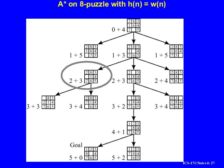
- 27. A* on 8-puzzle with h(n) = w(n)
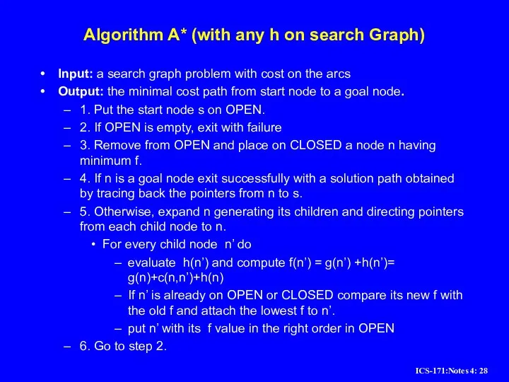
- 28. Algorithm A* (with any h on search Graph) Input: a search graph problem with cost on
- 29. S G A B D E C F 2 1 2 5 4 2 4 3
- 30. Example of A* Algorithm in action S A D B D C E E B F
- 31. Behavior of A* - Completeness Theorem (completeness for optimal solution) (HNL, 1968): If the heuristic function
- 33. Consistent heuristics A heuristic is consistent if for every node n, every successor n' of n
- 34. Optimality of A* with consistent h A* expands nodes in order of increasing f value Gradually
- 35. Summary: Consistent (Monotone) Heuristics If in the search graph the heuristic function satisfies triangle inequality for
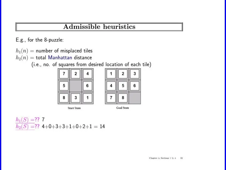
- 36. Admissible heuristics E.g., for the 8-puzzle: h1(n) = number of misplaced tiles h2(n) = total Manhattan
- 37. Admissible heuristics E.g., for the 8-puzzle: h1(n) = number of misplaced tiles h2(n) = total Manhattan
- 38. Dominance If h2(n) ≥ h1(n) for all n (both admissible) then h2 dominates h1 h2 is
- 39. Complexity of A* A* is optimally efficient (Dechter and Pearl 1985): It can be shown that
- 40. Effectiveness of A* Search Algorithm d IDS A*(h1) A*(h2) 2 10 6 6 4 112 13
- 41. Properties of A* Complete? Yes (unless there are infinitely many nodes with f ≤ f(G) )
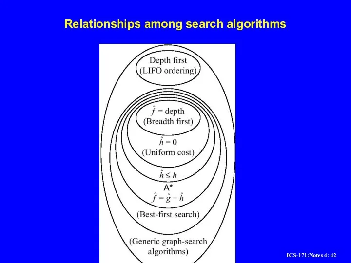
- 42. Relationships among search algorithms
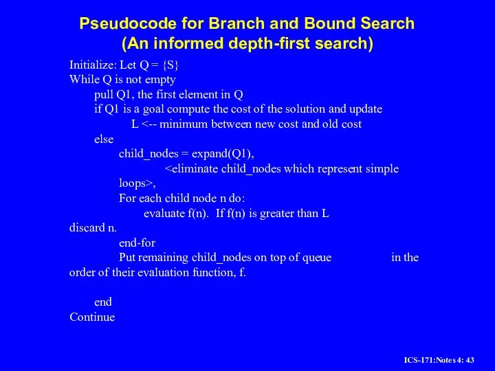
- 43. Pseudocode for Branch and Bound Search (An informed depth-first search) Initialize: Let Q = {S} While
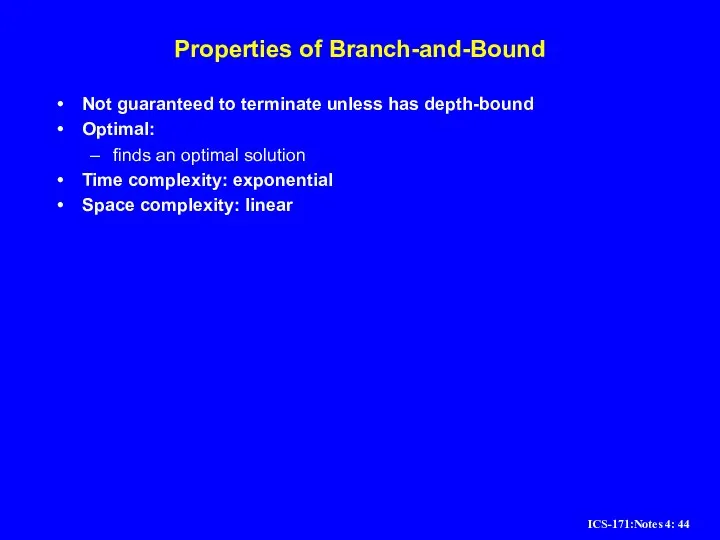
- 44. Properties of Branch-and-Bound Not guaranteed to terminate unless has depth-bound Optimal: finds an optimal solution Time
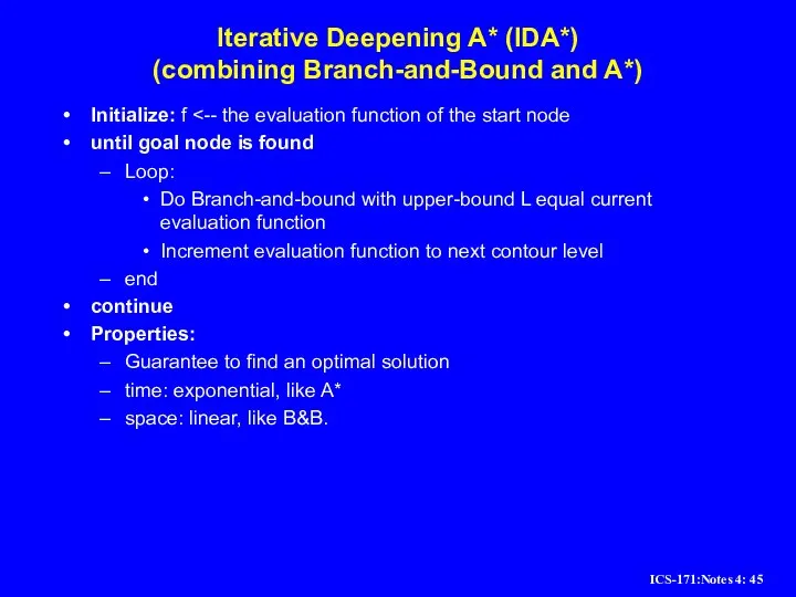
- 45. Iterative Deepening A* (IDA*) (combining Branch-and-Bound and A*) Initialize: f until goal node is found Loop:
- 47. Inventing Heuristics automatically Examples of Heuristic Functions for A* the 8-puzzle problem the number of tiles
- 48. Inventing Heuristics Automatically (continued) How did we find h1 and h2 for the 8-puzzle? verify admissibility?
- 49. Generating heuristics (continued) Example: TSP Finr a tour. A tour is: 1. A graph 2. Connected
- 50. Relaxed problems A problem with fewer restrictions on the actions is called a relaxed problem The
- 52. Automating Heuristic generation Use Strips representation: Operators: Pre-conditions, add-list, delete list 8-puzzle example: On(x,y), clear(y) adj(y,z)
- 53. Heuristic generation The space of relaxations can be enriched by predicate refinements Adj(y,z) iff neigbour(y,z) and
- 54. Improving Heuristics If we have several heuristics which are non dominating we can select the max
- 55. Local search algorithms In many optimization problems, the path to the goal is irrelevant; the goal
- 57. Hill-climbing search "Like climbing Everest in thick fog with amnesia"
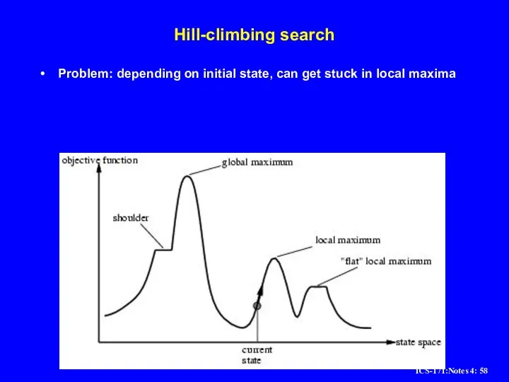
- 58. Hill-climbing search Problem: depending on initial state, can get stuck in local maxima
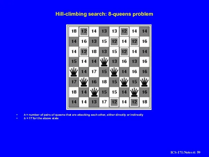
- 59. Hill-climbing search: 8-queens problem h = number of pairs of queens that are attacking each other,
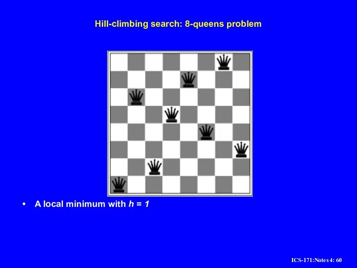
- 60. Hill-climbing search: 8-queens problem A local minimum with h = 1
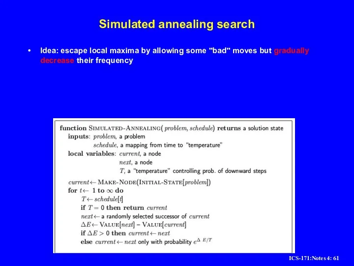
- 61. Simulated annealing search Idea: escape local maxima by allowing some "bad" moves but gradually decrease their
- 63. Скачать презентацию
Слайд 2Summary
Heuristics and Optimal search strategies
heuristics
hill-climbing algorithms
Best-First search
A*: optimal search using heuristics
Properties of
Summary
Heuristics and Optimal search strategies
heuristics
hill-climbing algorithms
Best-First search
A*: optimal search using heuristics
Properties of
Слайд 3Problem: finding a Minimum Cost Path
Previously we wanted an arbitrary path to
Problem: finding a Minimum Cost Path
Previously we wanted an arbitrary path to
Слайд 4Best-first search
Idea: use an evaluation function f(n) for each node
estimate of "desirability"
Expand
Best-first search
Idea: use an evaluation function f(n) for each node
estimate of "desirability"
Expand
Слайд 5Heuristic functions
8-puzzle
8-queen
Travelling salesperson
Heuristic functions
8-puzzle
8-queen
Travelling salesperson
Слайд 6Heuristic functions
8-puzzle
W(n): number of misplaced tiles
Manhatten distance
Gaschnig’s
8-queen
Travelling salesperson
Heuristic functions
8-puzzle
W(n): number of misplaced tiles
Manhatten distance
Gaschnig’s
8-queen
Travelling salesperson
Слайд 7Heuristic functions
8-puzzle
W(n): number of misplaced tiles
Manhatten distance
Gaschnig’s
8-queen
Number of future feasible slots
Min number
Heuristic functions
8-puzzle
W(n): number of misplaced tiles
Manhatten distance
Gaschnig’s
8-queen
Number of future feasible slots
Min number
Слайд 8Best first (Greedy) search: f(n) = number of misplaced tiles
Best first (Greedy) search: f(n) = number of misplaced tiles
Слайд 9Romania with step costs in km
Romania with step costs in km
Слайд 10Greedy best-first search
Evaluation function f(n) = h(n) (heuristic)
= estimate of cost from
Greedy best-first search
Evaluation function f(n) = h(n) (heuristic)
= estimate of cost from
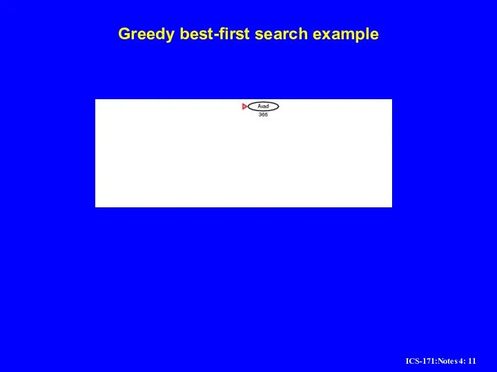
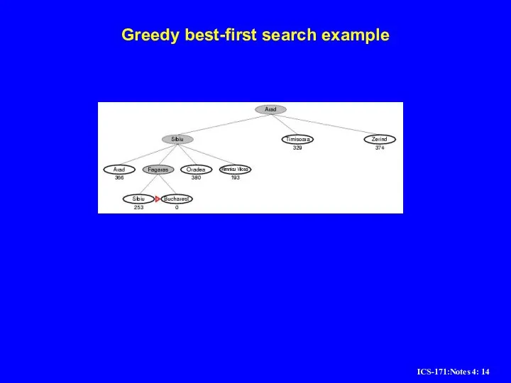
Слайд 11Greedy best-first search example
Greedy best-first search example
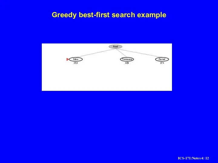
Слайд 12Greedy best-first search example
Greedy best-first search example
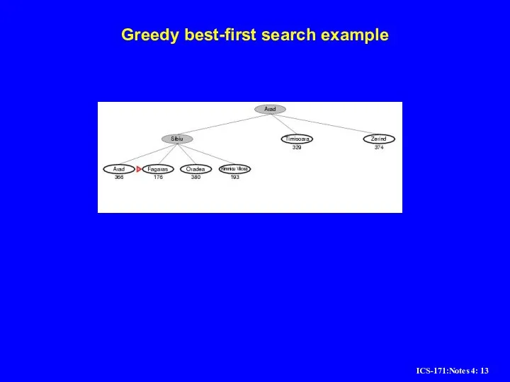
Слайд 13Greedy best-first search example
Greedy best-first search example
Слайд 14Greedy best-first search example
Greedy best-first search example
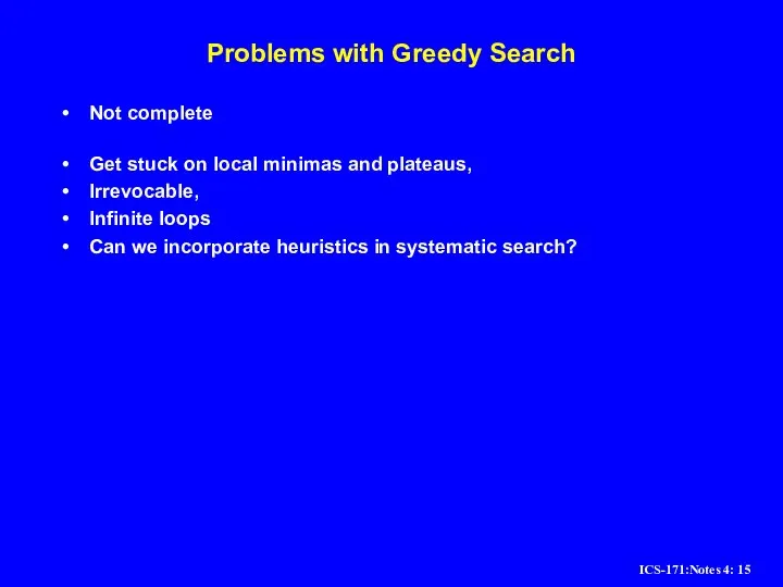
Слайд 15Problems with Greedy Search
Not complete
Get stuck on local minimas and plateaus,
Problems with Greedy Search
Not complete
Get stuck on local minimas and plateaus,
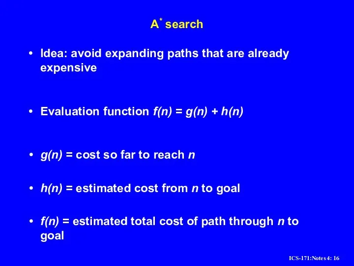
Слайд 16A* search
Idea: avoid expanding paths that are already expensive
Evaluation function f(n) =
A* search
Idea: avoid expanding paths that are already expensive
Evaluation function f(n) =
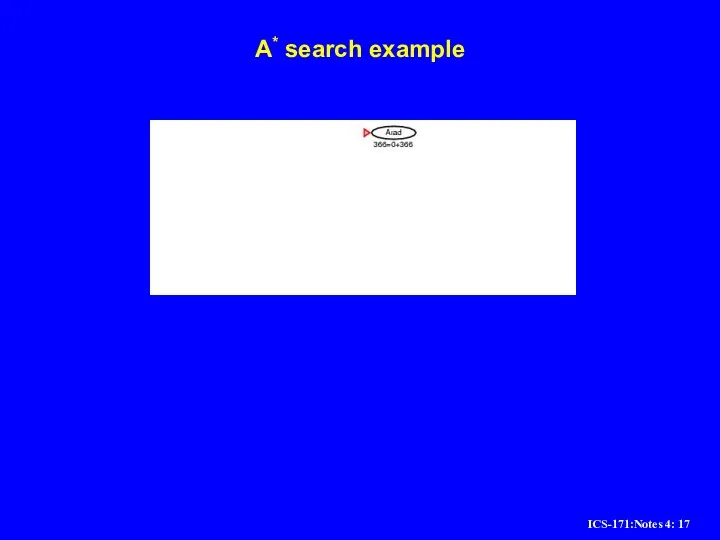
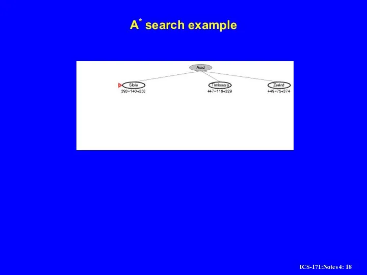
Слайд 17A* search example
A* search example
Слайд 18A* search example
A* search example
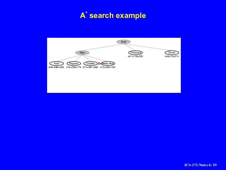
Слайд 19A* search example
A* search example
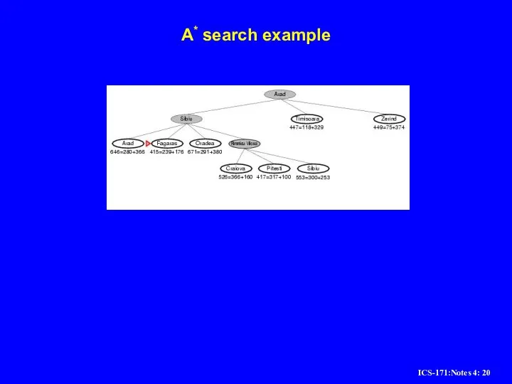
Слайд 20A* search example
A* search example
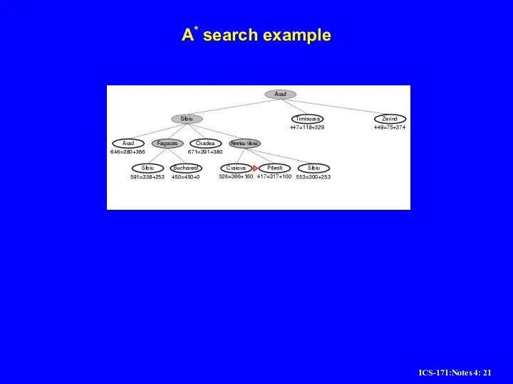
Слайд 21A* search example
A* search example
Слайд 22A* search example
A* search example
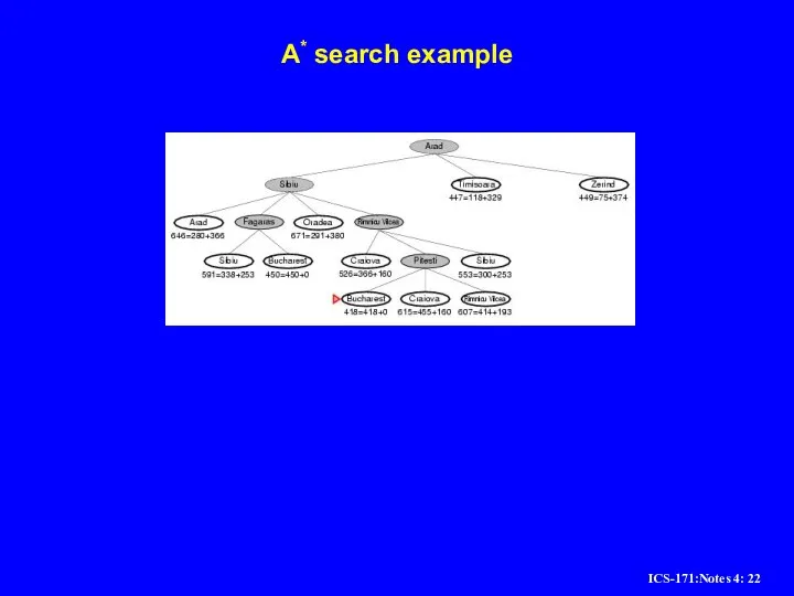
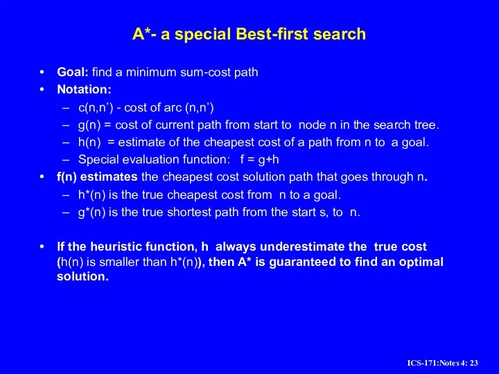
Слайд 23A*- a special Best-first search
Goal: find a minimum sum-cost path
Notation:
c(n,n’) - cost
A*- a special Best-first search
Goal: find a minimum sum-cost path
Notation:
c(n,n’) - cost
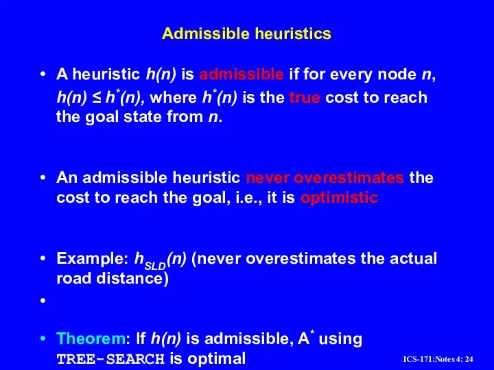
Слайд 24Admissible heuristics
A heuristic h(n) is admissible if for every node n,
h(n) ≤
Admissible heuristics
A heuristic h(n) is admissible if for every node n,
h(n) ≤
Слайд 27A* on 8-puzzle with h(n) = w(n)
A* on 8-puzzle with h(n) = w(n)
Слайд 28Algorithm A* (with any h on search Graph)
Input: a search graph problem
Algorithm A* (with any h on search Graph)
Input: a search graph problem
Слайд 29S
G
A
B
D
E
C
F
2
1
2
5
4
2
4
3
5
S
G
A
B
D
E
C
F
2
1
2
5
4
2
4
3
5
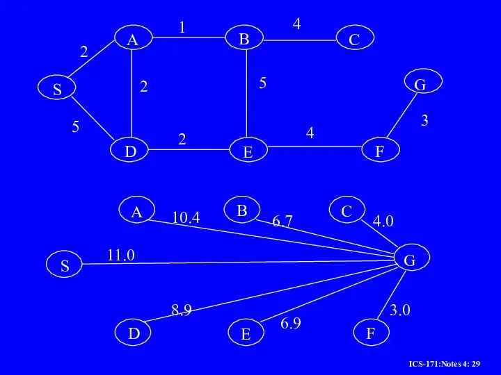
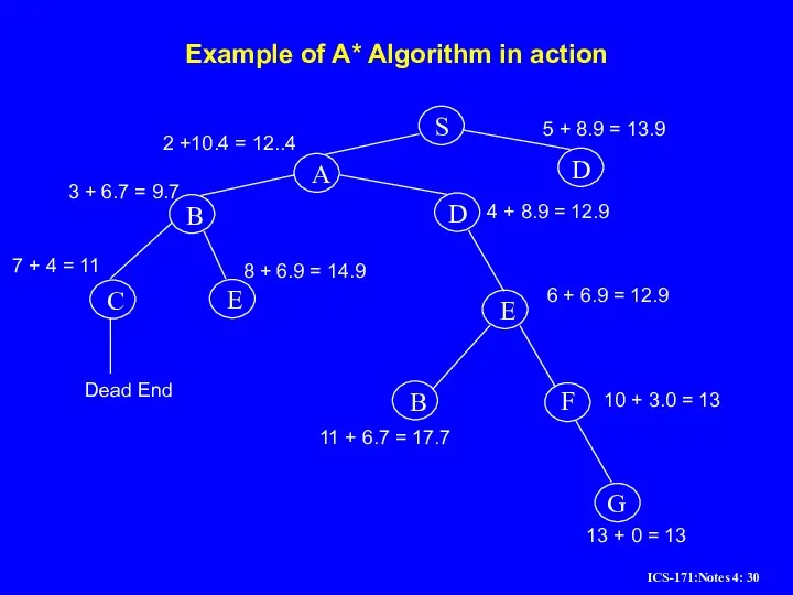
Слайд 30Example of A* Algorithm in action
S
A
D
B
D
C
E
E
B
F
G
2 +10.4 = 12..4
5 + 8.9 =
Example of A* Algorithm in action
S
A
D
B
D
C
E
E
B
F
G
2 +10.4 = 12..4
5 + 8.9 =
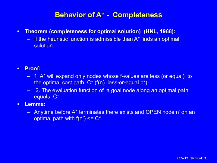
Слайд 31Behavior of A* - Completeness
Theorem (completeness for optimal solution) (HNL, 1968):
If
Behavior of A* - Completeness
Theorem (completeness for optimal solution) (HNL, 1968):
If
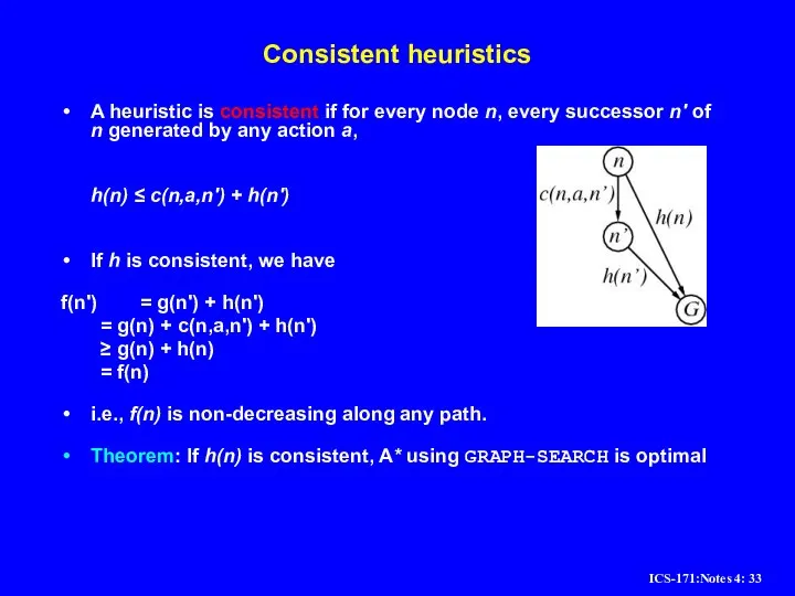
Слайд 33Consistent heuristics
A heuristic is consistent if for every node n, every successor
Consistent heuristics
A heuristic is consistent if for every node n, every successor
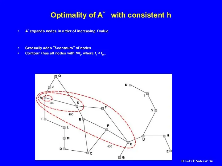
Слайд 34Optimality of A* with consistent h
A* expands nodes in order of increasing
Optimality of A* with consistent h
A* expands nodes in order of increasing
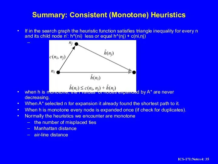
Слайд 35Summary: Consistent (Monotone) Heuristics
If in the search graph the heuristic function satisfies
Summary: Consistent (Monotone) Heuristics
If in the search graph the heuristic function satisfies
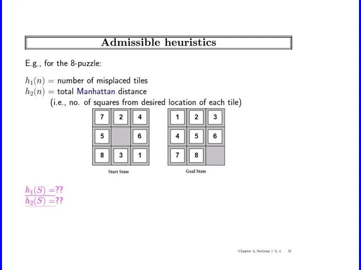
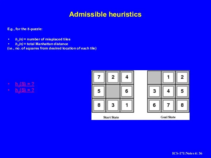
Слайд 36Admissible heuristics
E.g., for the 8-puzzle:
h1(n) = number of misplaced tiles
h2(n) = total
Admissible heuristics
E.g., for the 8-puzzle:
h1(n) = number of misplaced tiles
h2(n) = total
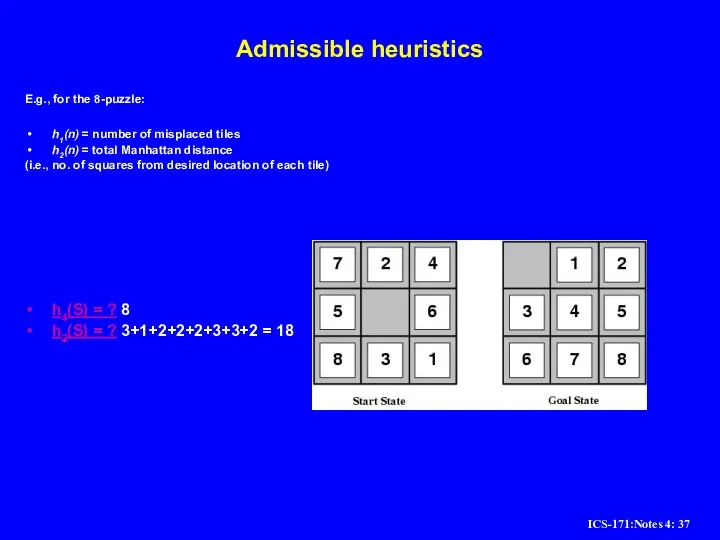
Слайд 37Admissible heuristics
E.g., for the 8-puzzle:
h1(n) = number of misplaced tiles
h2(n) = total
Admissible heuristics
E.g., for the 8-puzzle:
h1(n) = number of misplaced tiles
h2(n) = total
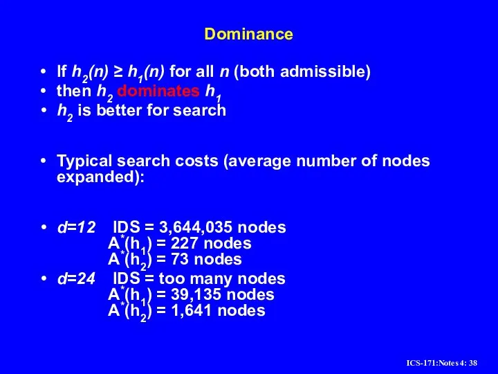
Слайд 38Dominance
If h2(n) ≥ h1(n) for all n (both admissible)
then h2 dominates h1
Dominance
If h2(n) ≥ h1(n) for all n (both admissible)
then h2 dominates h1
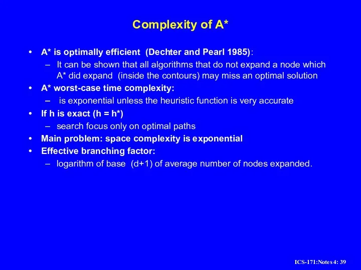
Слайд 39Complexity of A*
A* is optimally efficient (Dechter and Pearl 1985):
It can be
Complexity of A*
A* is optimally efficient (Dechter and Pearl 1985):
It can be
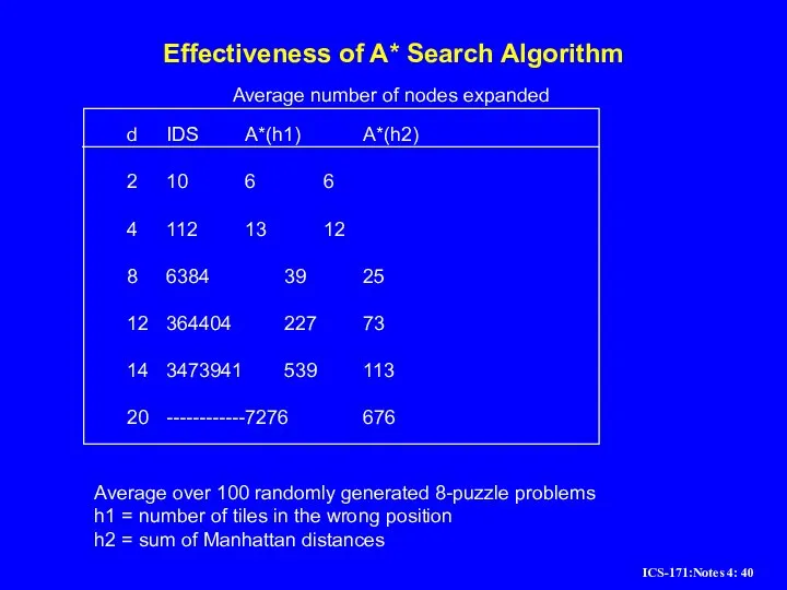
Слайд 40Effectiveness of A* Search Algorithm
d IDS A*(h1) A*(h2)
2 10 6 6
4 112 13 12
8 6384 39 25
12 364404 227 73
14 3473941 539 113
20 ------------ 7276 676
Average number of nodes expanded
Average over 100 randomly
Effectiveness of A* Search Algorithm
d IDS A*(h1) A*(h2)
2 10 6 6
4 112 13 12
8 6384 39 25
12 364404 227 73
14 3473941 539 113
20 ------------ 7276 676
Average number of nodes expanded
Average over 100 randomly
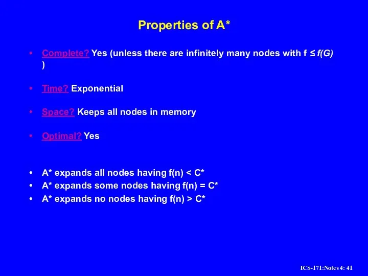
Слайд 41Properties of A*
Complete? Yes (unless there are infinitely many nodes with f
Properties of A*
Complete? Yes (unless there are infinitely many nodes with f
Слайд 42Relationships among search algorithms
Relationships among search algorithms
Слайд 43Pseudocode for Branch and Bound Search
(An informed depth-first search)
Initialize: Let Q =
Pseudocode for Branch and Bound Search
(An informed depth-first search)
Initialize: Let Q =
Слайд 44Properties of Branch-and-Bound
Not guaranteed to terminate unless has depth-bound
Optimal:
finds an optimal
Properties of Branch-and-Bound
Not guaranteed to terminate unless has depth-bound
Optimal:
finds an optimal
Слайд 45Iterative Deepening A* (IDA*)
(combining Branch-and-Bound and A*)
Initialize: f <-- the evaluation function
Iterative Deepening A* (IDA*)
(combining Branch-and-Bound and A*)
Initialize: f <-- the evaluation function
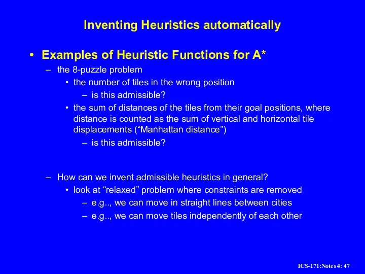
Слайд 47Inventing Heuristics automatically
Examples of Heuristic Functions for A*
the 8-puzzle problem
the number of
Inventing Heuristics automatically
Examples of Heuristic Functions for A*
the 8-puzzle problem
the number of
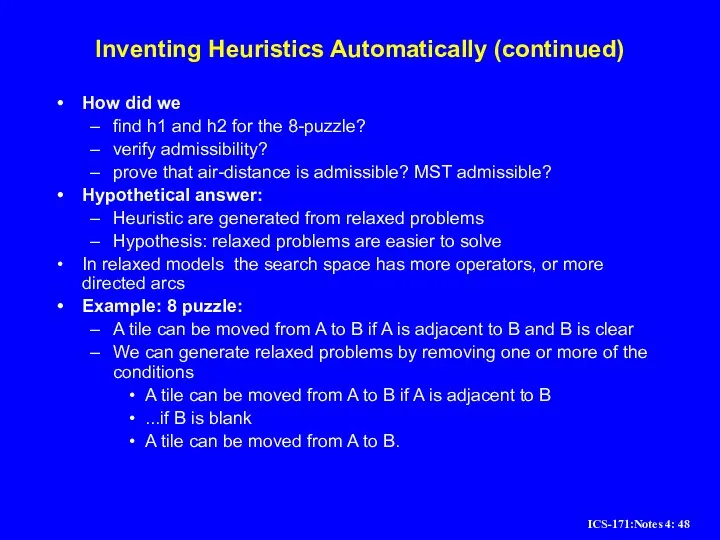
Слайд 48Inventing Heuristics Automatically (continued)
How did we
find h1 and h2 for the
Inventing Heuristics Automatically (continued)
How did we
find h1 and h2 for the
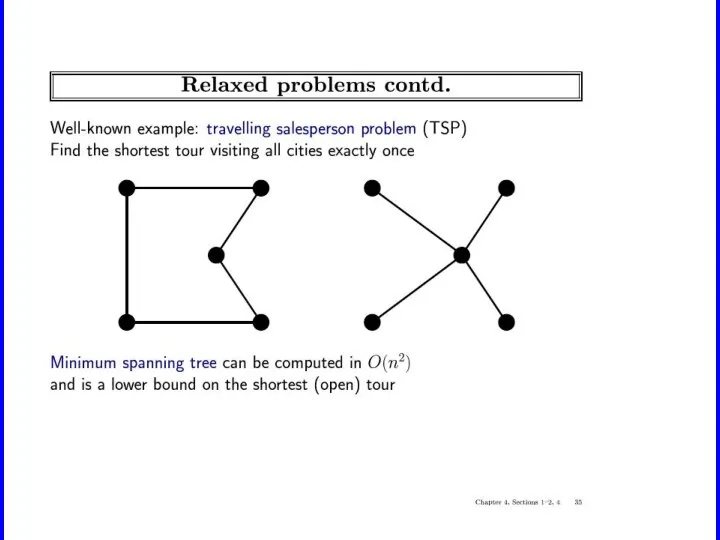
Слайд 49Generating heuristics (continued)
Example: TSP
Finr a tour. A tour is:
1. A graph
2. Connected
3.
Generating heuristics (continued)
Example: TSP
Finr a tour. A tour is:
1. A graph
2. Connected
3.
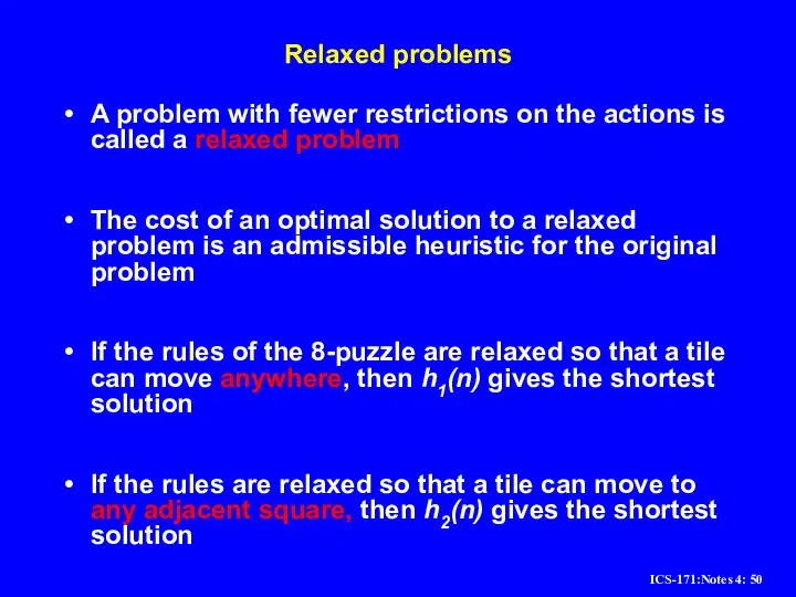
Слайд 50Relaxed problems
A problem with fewer restrictions on the actions is called a
Relaxed problems
A problem with fewer restrictions on the actions is called a
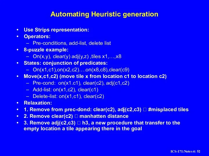
Слайд 52Automating Heuristic generation
Use Strips representation:
Operators:
Pre-conditions, add-list, delete list
8-puzzle example:
On(x,y), clear(y) adj(y,z) ,tiles
Automating Heuristic generation
Use Strips representation:
Operators:
Pre-conditions, add-list, delete list
8-puzzle example:
On(x,y), clear(y) adj(y,z) ,tiles
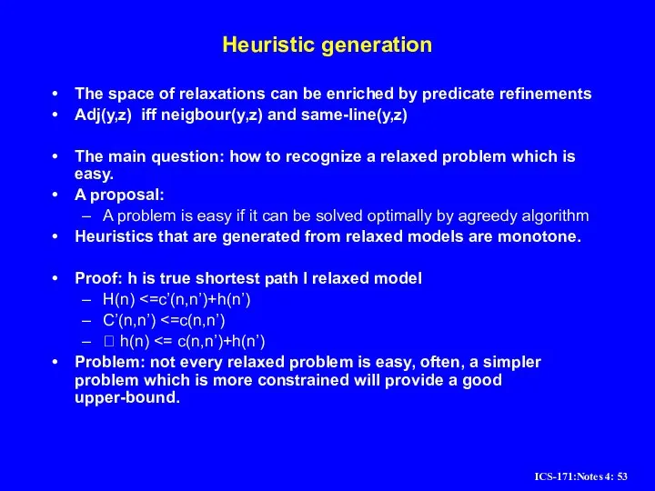
Слайд 53Heuristic generation
The space of relaxations can be enriched by predicate refinements
Adj(y,z) iff
Heuristic generation
The space of relaxations can be enriched by predicate refinements
Adj(y,z) iff
Слайд 54Improving Heuristics
If we have several heuristics which are non dominating we can
Improving Heuristics
If we have several heuristics which are non dominating we can
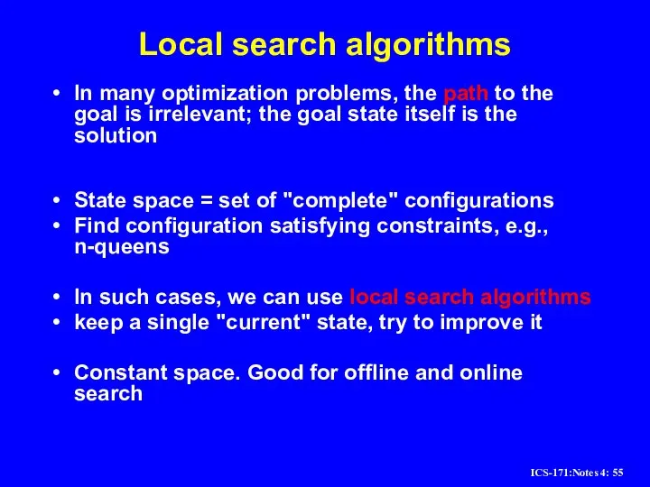
Слайд 55Local search algorithms
In many optimization problems, the path to the goal is
Local search algorithms
In many optimization problems, the path to the goal is
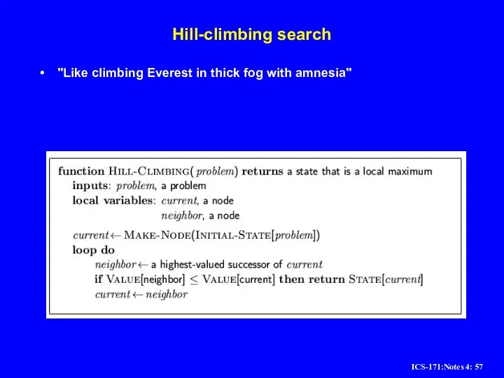
Слайд 57Hill-climbing search
"Like climbing Everest in thick fog with amnesia"
Hill-climbing search
"Like climbing Everest in thick fog with amnesia"
Слайд 58Hill-climbing search
Problem: depending on initial state, can get stuck in local maxima
Hill-climbing search
Problem: depending on initial state, can get stuck in local maxima
Слайд 59Hill-climbing search: 8-queens problem
h = number of pairs of queens that are
Hill-climbing search: 8-queens problem
h = number of pairs of queens that are
Слайд 60Hill-climbing search: 8-queens problem
A local minimum with h = 1
Hill-climbing search: 8-queens problem
A local minimum with h = 1
Слайд 61Simulated annealing search
Idea: escape local maxima by allowing some "bad" moves but
Simulated annealing search
Idea: escape local maxima by allowing some "bad" moves but
 Лицеисты
 Техника прыжка в длину с места
 The best job in the world
  Проект «Протяни руку детству»
 Шаблон АУЭС
 Простые механизмы. Рычаг. Условие равновесия рычага. Применение рычага, блока, наклонной плоскости
 Творчество
 New Zealand
 Документы для регистрации аттракциона
 Контекстный баннер
 Гипотеза
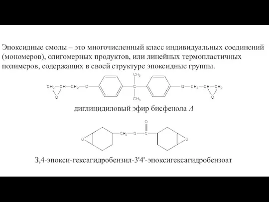 технология получения эпоксидных смол
 Алгоритмы
 Где ума набраться…
 Как правильно чистить зубы
 Темы 2.1 и 2.2. Организация и схема проведения внешнеэкономической операции при прямых и косвенных связях между контрагентами. Орган
 Introduction to Civil law
 Всероссийская патриотическая акция Снежный десант РСО
 Основные задачи на проценты
 Презентация на тему Река Дон
 Опыт использования AbsOPAC для обслуживания читателей в МПГУ
 , = (1 класс)">Равенства. Неравенства. Знаки
 新款敬请后续保持关注
 Технические средства в сфере строительства
 Начало третьего дня профполигона. Трениг Бизнес – моделирование
 Репрезнтативные системы
 УПРАВЛЕНИЕ КАЧЕСТВОМ
 Самые страшные тюрьмы России и мира