- Neural Networks

Содержание
- 2. Pachshenko Galina Nikolaevna Associate Professor of Information System Department, Candidate of Technical Science
- 3. Week 7 Lecture 7
- 4. Topics Types of Optimization Algorithms used in Neural Networks Gradient descent
- 5. Have you ever wondered which optimization algorithm to use for your Neural network Model to produce
- 6. What are Optimization Algorithms ?
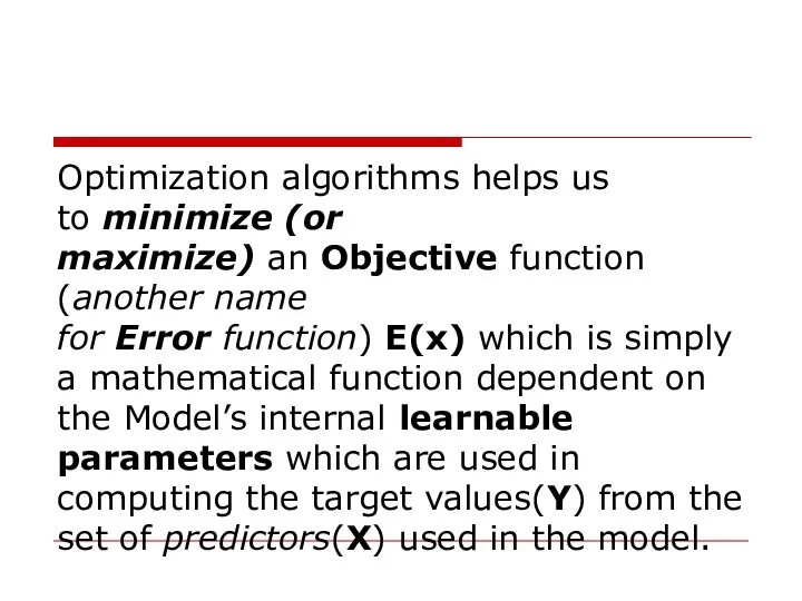
- 7. Optimization algorithms helps us to minimize (or maximize) an Objective function (another name for Error function)
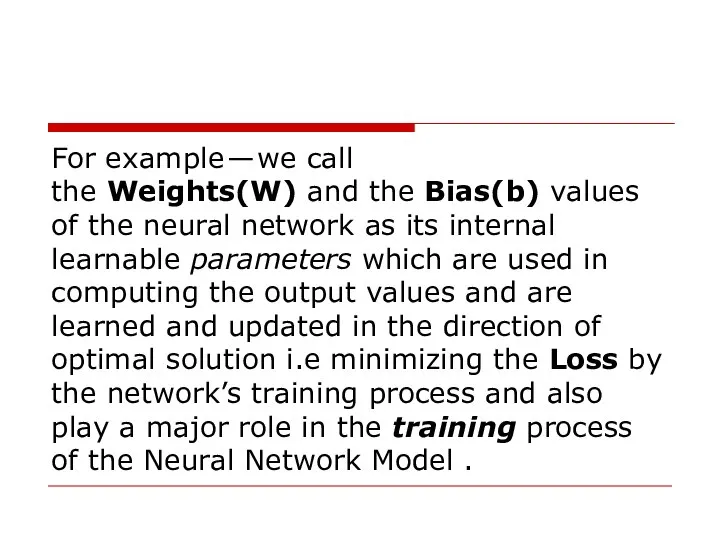
- 8. For example — we call the Weights(W) and the Bias(b) values of the neural network as
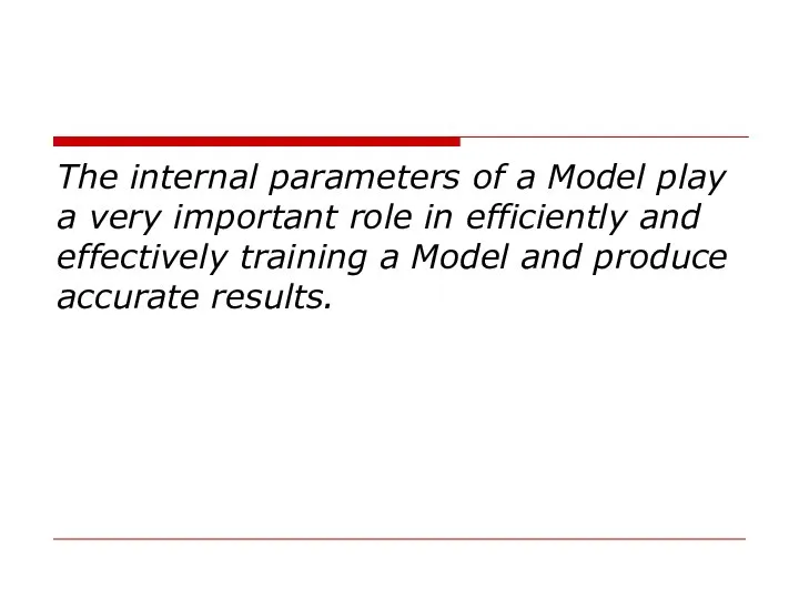
- 9. The internal parameters of a Model play a very important role in efficiently and effectively training
- 10. This is why we use various Optimization strategies and algorithms to update and calculate appropriate and
- 11. Optimization Algorithm falls in 2 major categories
- 12. First Order Optimization Algorithms — These algorithms minimize or maximize a Loss function E(x) using its
- 13. The First order derivative tells us whether the function is decreasing or increasing at a particular
- 14. What is a Gradient of a function?
- 15. A Gradient is simply a vector which is a multi-variable generalization of a derivative(dy/dx) which is
- 16. The difference is that to calculate a derivative of a function which is dependent on more
- 17. A Gradient is represented by a Jacobian Matrix — which is simply a Matrix consisting of
- 18. Hence summing up, a derivative is simply defined for a function dependent on single variables ,
- 19. Second Order Optimization Algorithms — Second-order methods use the second order derivative which is also called
- 20. The Hessian is a Matrix of Second Order Partial Derivatives. Since the second derivative is costly
- 21. The second order derivative tells us whether the first derivative is increasing or decreasing which hints
- 22. Some Advantages of Second Order Optimization over First Order — Although the Second Order Derivative may
- 23. What are the different types of Optimization Algorithms used in Neural Networks ?
- 24. Gradient Descent Variants of Gradient Descent: Batch Gradient Descent; Stochastic gradient descent; Mini Batch Gradient Descent
- 25. Gradient Descent is the most important technique and the foundation of how we train and optimize
- 26. “Gradient Descent — Find the Minima , control the variance and then update the Model’s parameters
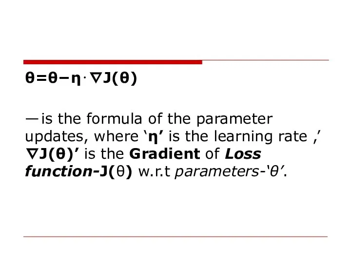
- 27. θ=θ−η⋅∇J(θ) — is the formula of the parameter updates, where ‘η’ is the learning rate ,’∇J(θ)’
- 28. The parameter η is the training rate. This value can either set to a fixed value
- 29. It is the most popular Optimization algorithms used in optimizing a Neural Network. Now gradient descent
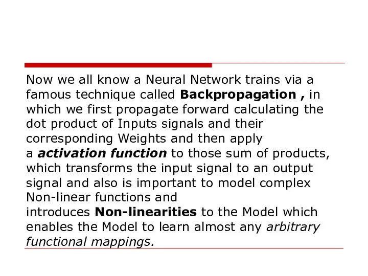
- 30. Now we all know a Neural Network trains via a famous technique called Backpropagation , in
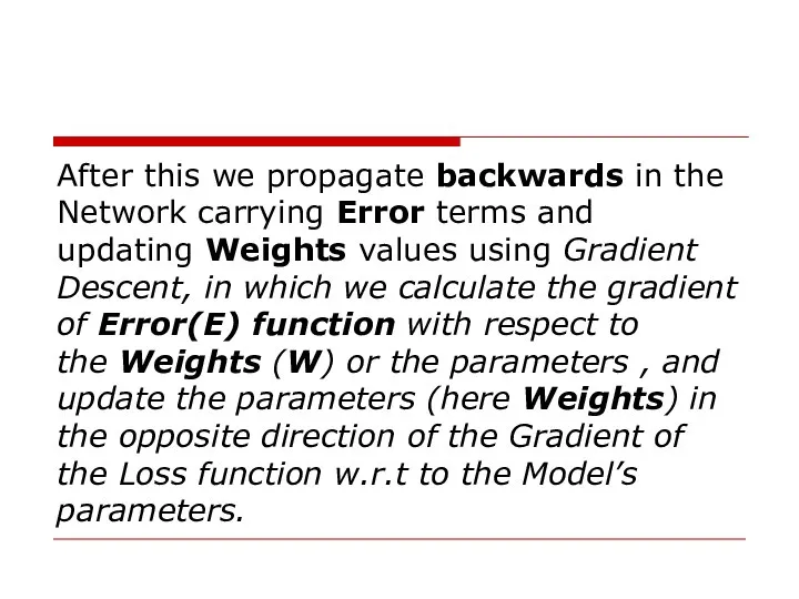
- 31. After this we propagate backwards in the Network carrying Error terms and updating Weights values using
- 33. The image on above shows the process of Weight updates in the opposite direction of the
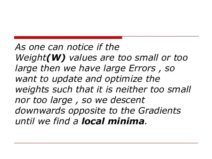
- 34. As one can notice if the Weight(W) values are too small or too large then we
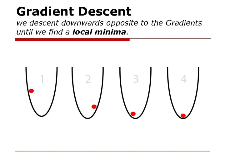
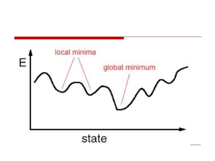
- 35. Gradient Descent we descent downwards opposite to the Gradients until we find a local minima.
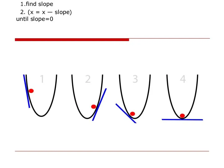
- 36. 1.find slope 2. (x = x — slope) until slope=0
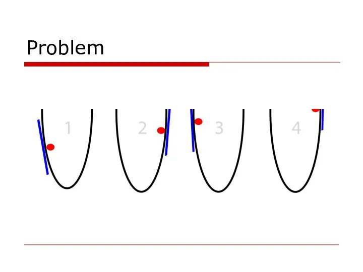
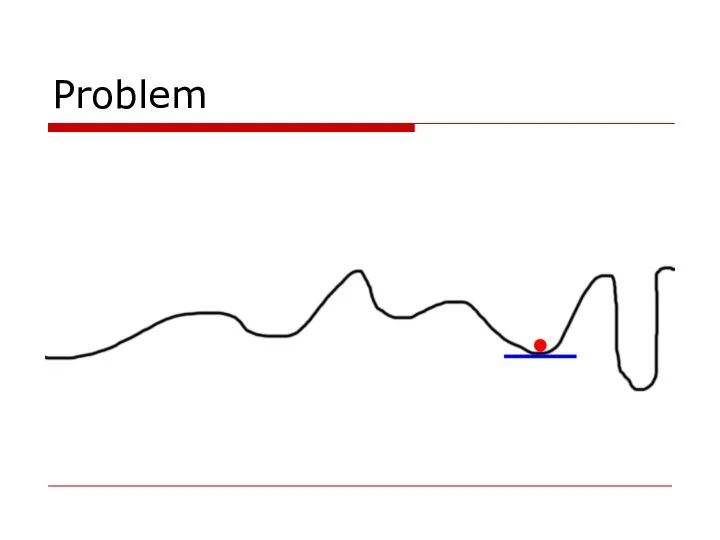
- 37. Problem
- 38. 1. find slope 2. alpha = 0.1 (or any number from 0 to 1) 3. x
- 39. Problem
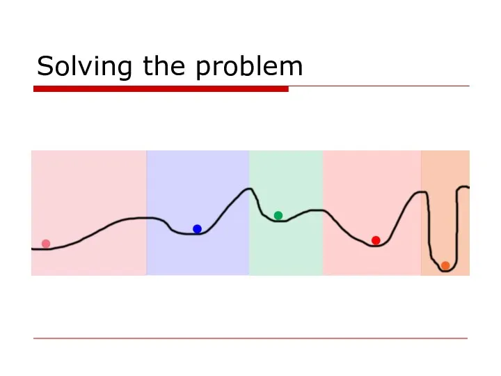
- 41. Solving the problem
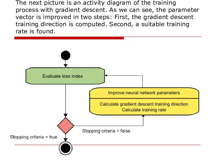
- 42. The next picture is an activity diagram of the training process with gradient descent. As we
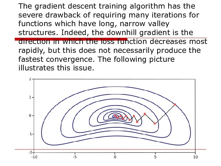
- 43. The gradient descent training algorithm has the severe drawback of requiring many iterations for functions which
- 44. Gradient descent is the recommended algorithm when we have very big neural networks, with many thousand
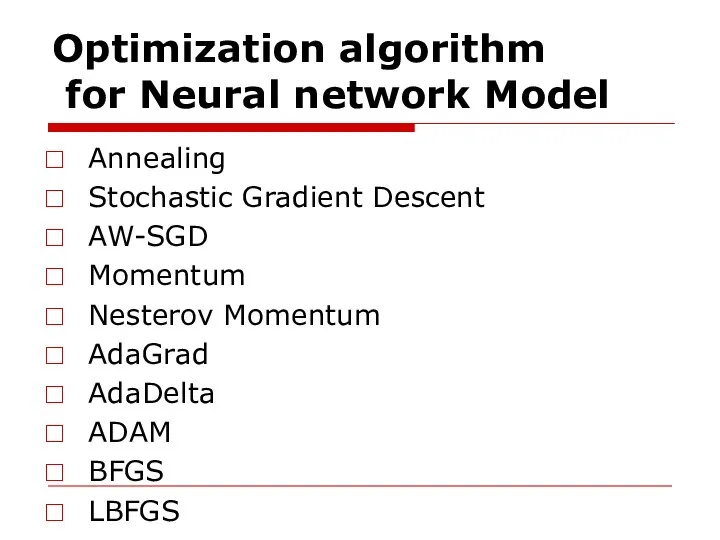
- 45. Optimization algorithm for Neural network Model Annealing Stochastic Gradient Descent AW-SGD Momentum Nesterov Momentum AdaGrad AdaDelta
- 47. Скачать презентацию
Слайд 3Week 7
Lecture 7
Week 7
Lecture 7
Слайд 4Topics
Types of Optimization Algorithms used in Neural Networks
Gradient descent
Topics
Types of Optimization Algorithms used in Neural Networks
Gradient descent
Слайд 5Have you ever wondered which optimization algorithm to use for your Neural
Have you ever wondered which optimization algorithm to use for your Neural
Слайд 6What are Optimization Algorithms ?
What are Optimization Algorithms ?
Слайд 7Optimization algorithms helps us to minimize (or maximize) an Objective function (another name for Error function) E(x) which is
Optimization algorithms helps us to minimize (or maximize) an Objective function (another name for Error function) E(x) which is
Слайд 8For example — we call the Weights(W) and the Bias(b) values of the neural network as its internal
For example — we call the Weights(W) and the Bias(b) values of the neural network as its internal
Слайд 9The internal parameters of a Model play a very important role in
The internal parameters of a Model play a very important role in
Слайд 10This is why we use various Optimization strategies and algorithms to update
This is why we use various Optimization strategies and algorithms to update
Слайд 11Optimization Algorithm falls in 2 major categories
Optimization Algorithm falls in 2 major categories
Слайд 12First Order Optimization Algorithms — These algorithms minimize or maximize a Loss function E(x) using its Gradient values
First Order Optimization Algorithms — These algorithms minimize or maximize a Loss function E(x) using its Gradient values
Слайд 13The First order derivative tells us whether the function is decreasing or
The First order derivative tells us whether the function is decreasing or
Слайд 14What is a Gradient of a function?
What is a Gradient of a function?
Слайд 15A Gradient is simply a vector which is a multi-variable generalization of a derivative(dy/dx) which
A Gradient is simply a vector which is a multi-variable generalization of a derivative(dy/dx) which
Слайд 16The difference is that to calculate a derivative of a function which
The difference is that to calculate a derivative of a function which
Слайд 17A Gradient is represented by a Jacobian Matrix — which is simply a Matrix consisting of first order partial
A Gradient is represented by a Jacobian Matrix — which is simply a Matrix consisting of first order partial
Слайд 18Hence summing up, a derivative is simply defined for a function dependent
Hence summing up, a derivative is simply defined for a function dependent
Слайд 19Second Order Optimization Algorithms — Second-order methods use the second order derivative which is also called Hessian to
Second Order Optimization Algorithms — Second-order methods use the second order derivative which is also called Hessian to
Слайд 20The Hessian is a Matrix of Second Order Partial Derivatives. Since the second derivative is costly
The Hessian is a Matrix of Second Order Partial Derivatives. Since the second derivative is costly
Слайд 21The second order derivative tells us whether the first derivative is increasing or decreasing
The second order derivative tells us whether the first derivative is increasing or decreasing
Слайд 22Some Advantages of Second Order Optimization over First Order —
Although the Second Order
Some Advantages of Second Order Optimization over First Order —
Although the Second Order
Слайд 23What are the different types of Optimization Algorithms used in Neural Networks ?
What are the different types of Optimization Algorithms used in Neural Networks ?
Слайд 24Gradient Descent
Variants of Gradient Descent: Batch Gradient Descent; Stochastic gradient descent; Mini Batch Gradient Descent
Gradient Descent
Variants of Gradient Descent: Batch Gradient Descent; Stochastic gradient descent; Mini Batch Gradient Descent
Слайд 25Gradient Descent is the most important technique and the foundation of how we
Gradient Descent is the most important technique and the foundation of how we
Слайд 26“Gradient Descent — Find the Minima , control the variance and then update the Model’s
“Gradient Descent — Find the Minima , control the variance and then update the Model’s
Слайд 27θ=θ−η⋅∇J(θ)
— is the formula of the parameter updates, where ‘η’ is the learning rate ,’∇J(θ)’ is
θ=θ−η⋅∇J(θ)
— is the formula of the parameter updates, where ‘η’ is the learning rate ,’∇J(θ)’ is
Слайд 28The parameter η is the training rate. This value can either set
The parameter η is the training rate. This value can either set
Слайд 29It is the most popular Optimization algorithms used in optimizing a Neural
It is the most popular Optimization algorithms used in optimizing a Neural
Слайд 30Now we all know a Neural Network trains via a famous technique
Now we all know a Neural Network trains via a famous technique
Слайд 31After this we propagate backwards in the Network carrying Error terms and updating Weights values using Gradient Descent, in
After this we propagate backwards in the Network carrying Error terms and updating Weights values using Gradient Descent, in
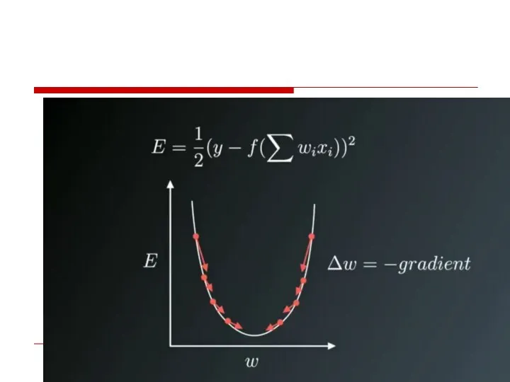
Слайд 33The image on above shows the process of Weight updates in the
The image on above shows the process of Weight updates in the
Слайд 34As one can notice if the Weight(W) values are too small or too
As one can notice if the Weight(W) values are too small or too
Слайд 35Gradient Descent
we descent downwards opposite to the Gradients until we find a local
Gradient Descent we descent downwards opposite to the Gradients until we find a local
Слайд 36 1.find slope
2. (x = x — slope)
until slope=0
1.find slope
2. (x = x — slope)
until slope=0
Слайд 37Problem
Problem
Слайд 381. find slope
2. alpha = 0.1 (or any number from 0
1. find slope 2. alpha = 0.1 (or any number from 0

Слайд 39Problem
Problem
Слайд 41Solving the problem
Solving the problem
Слайд 42The next picture is an activity diagram of the training process with
The next picture is an activity diagram of the training process with
Слайд 43The gradient descent training algorithm has the severe drawback of requiring many
The gradient descent training algorithm has the severe drawback of requiring many
Слайд 44Gradient descent is the recommended algorithm when we have very big neural
Gradient descent is the recommended algorithm when we have very big neural
Слайд 45Optimization algorithm
for Neural network Model
Annealing
Stochastic Gradient Descent
AW-SGD
Momentum
Nesterov Momentum
AdaGrad
AdaDelta
ADAM
BFGS
LBFGS
Optimization algorithm
for Neural network Model
Annealing
Stochastic Gradient Descent
AW-SGD
Momentum
Nesterov Momentum
AdaGrad
AdaDelta
ADAM
BFGS
LBFGS
 ПОРТФОЛИО ВОСПИТАТЕЛЯ
 Презентация на тему Минойская цивилизация
  PHIL 1- Lecture 3 - Week 3 moodle
 Железнодорожный тоннель
 FINANCIAL ANALYSIS AND
 Использование проектной методики в обучении иностранному языку
 Система права
 Гигиена питания
 Гигиена коз и овец
 Использование ФЦИОР на уроках физики
 Налоговый вычет по ценным бумагам
 Доли федеральных телеканалов при национальном и региональном размещении рекламы
 Презентация WasteVEM процесса
 Фея Флора. Богиня цветов и весны. С приходом весны властвовала над всеми живыми существами. Имя образовано от flos ("цветок"). По леген
 Старшов Петр Павлович
 Классицизм в литературе
 Методическая тема
 He’s. She
 Программа коррекции синдрова эмоционального выгорания и повышения стрессоустойчивости личности
 Пирог Ленивец
 Учебный семинар «Формирование универсальных учебных действий на уроках в начальной школе»
 Диалог о вредной привычке.
 Права та обовязки споживачів
 Mother teresa
 Удаление третьих моляров верхней и нижней челюсти. Ретенция и дистопия зубов мудрости
 Мыс өндіріс қалдықтарынан түсті металл тұздарын алуды жобалау
 Персональное предложение по регистрации товарного знака Баранкино для ИП (ООО) Под ключ
 Семь дней недели