- Project Analysis and Evaluation

Содержание
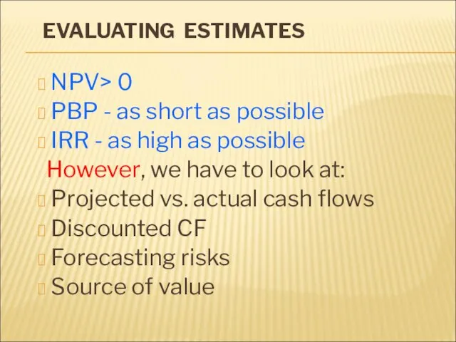
- 2. EVALUATING ESTIMATES NPV> 0 PBP - as short as possible IRR - as high as possible
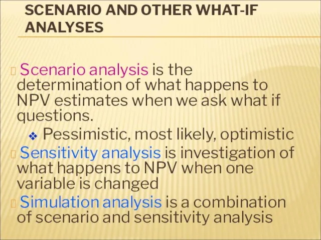
- 3. SCENARIO AND OTHER WHAT-IF ANALYSES Scenario analysis is the determination of what happens to NPV estimates
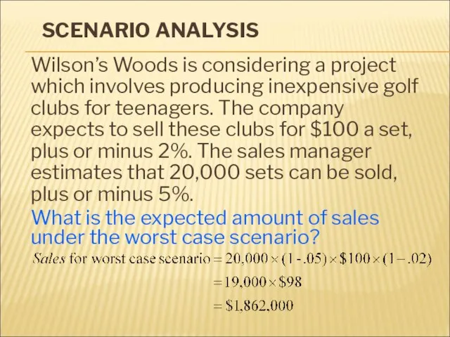
- 4. SCENARIO ANALYSIS Wilson’s Woods is considering a project which involves producing inexpensive golf clubs for teenagers.
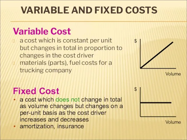
- 5. VARIABLE AND FIXED COSTS Variable Cost a cost which is constant per unit but changes in
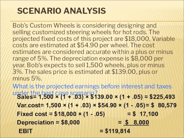
- 6. SCENARIO ANALYSIS Bob’s Custom Wheels is considering designing and selling customized steering wheels for hot rods.
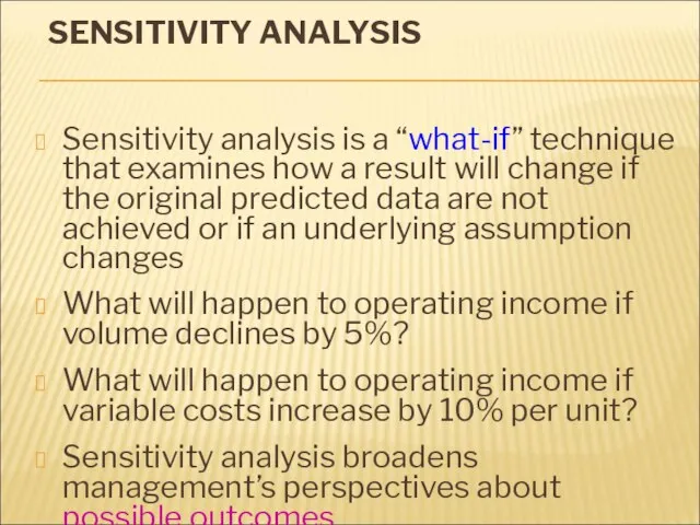
- 7. SENSITIVITY ANALYSIS Sensitivity analysis is a “what-if” technique that examines how a result will change if
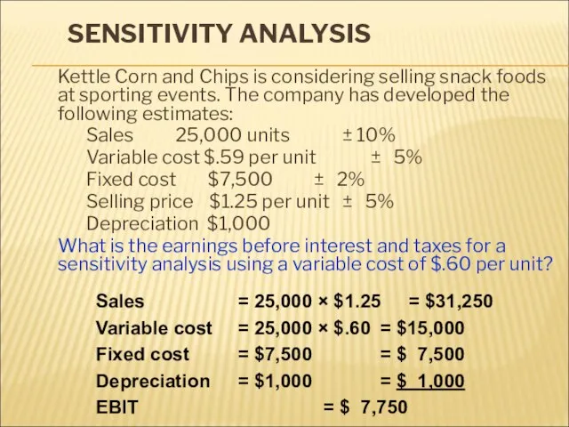
- 8. SENSITIVITY ANALYSIS Kettle Corn and Chips is considering selling snack foods at sporting events. The company
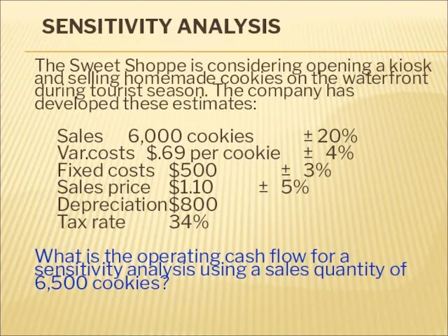
- 9. SENSITIVITY ANALYSIS The Sweet Shoppe is considering opening a kiosk and selling homemade cookies on the
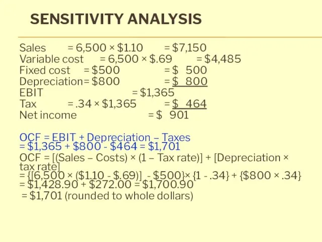
- 10. SENSITIVITY ANALYSIS Sales = 6,500 × $1.10 = $7,150 Variable cost = 6,500 × $.69 =
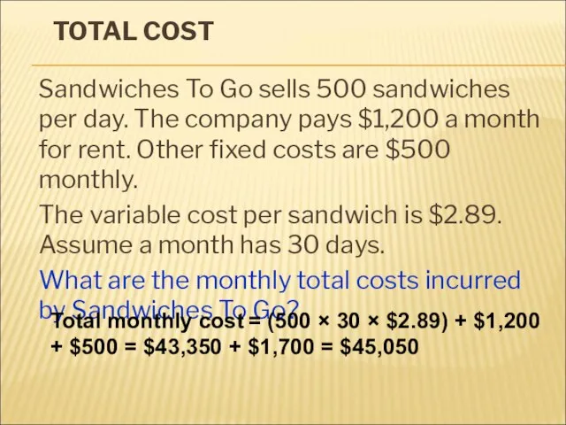
- 11. TOTAL COST Sandwiches To Go sells 500 sandwiches per day. The company pays $1,200 a month
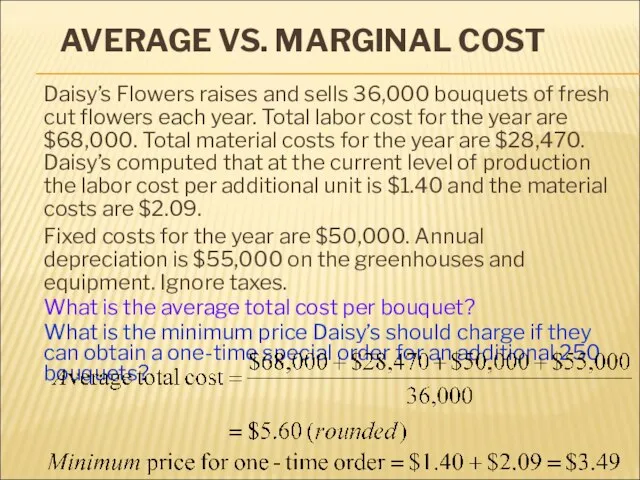
- 12. AVERAGE VS. MARGINAL COST Daisy’s Flowers raises and sells 36,000 bouquets of fresh cut flowers each
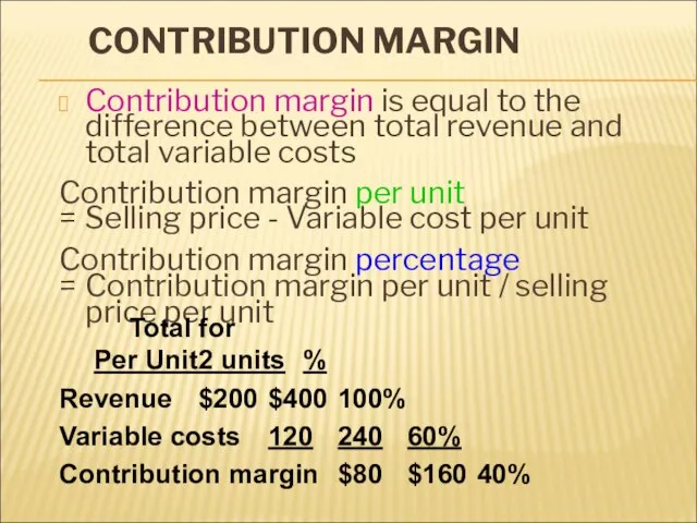
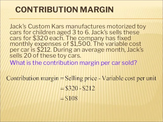
- 13. CONTRIBUTION MARGIN Contribution margin is equal to the difference between total revenue and total variable costs
- 14. CONTRIBUTION MARGIN Jack’s Custom Kars manufactures motorized toy cars for children aged 3 to 6. Jack’s
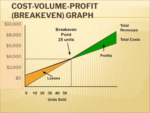
- 15. COST-VOLUME-PROFIT (BREAKEVEN) GRAPH $10,000 $8,000 $6,000 $4,000 $2,000 $0 0 10 20 30 40 50 Units
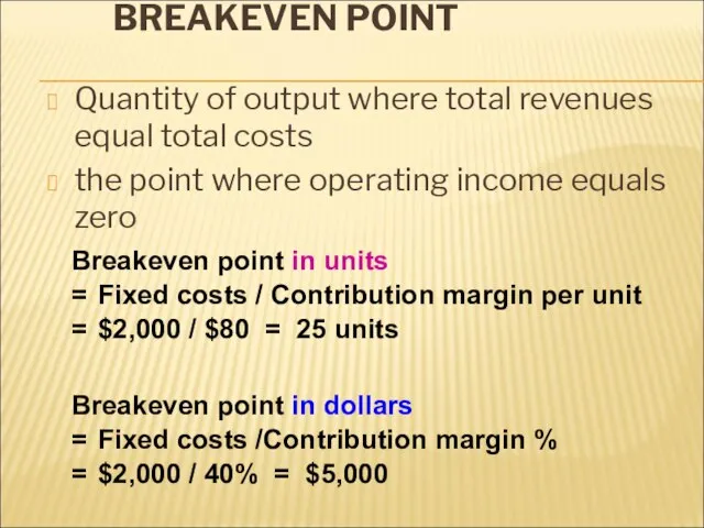
- 16. BREAKEVEN POINT Quantity of output where total revenues equal total costs the point where operating income
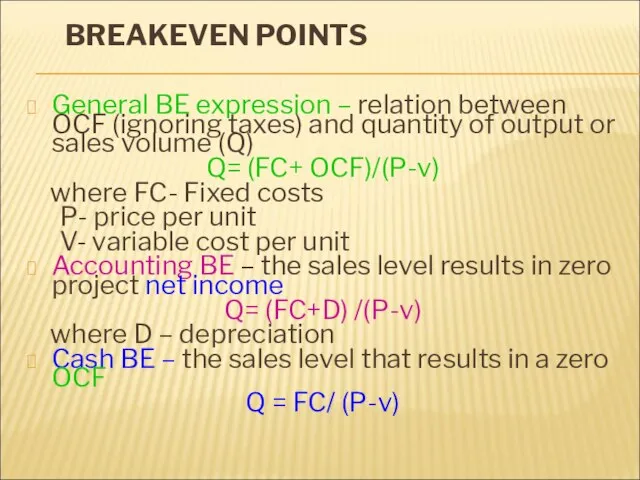
- 17. BREAKEVEN POINTS General BE expression – relation between OCF (ignoring taxes) and quantity of output or
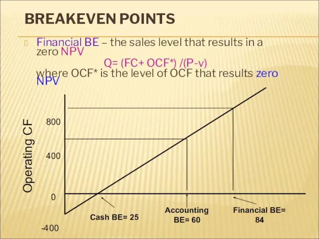
- 18. BREAKEVEN POINTS Financial BE – the sales level that results in a zero NPV Q= (FC+
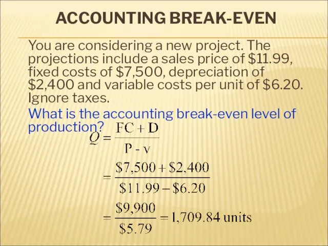
- 19. ACCOUNTING BREAK-EVEN You are considering a new project. The projections include a sales price of $11.99,
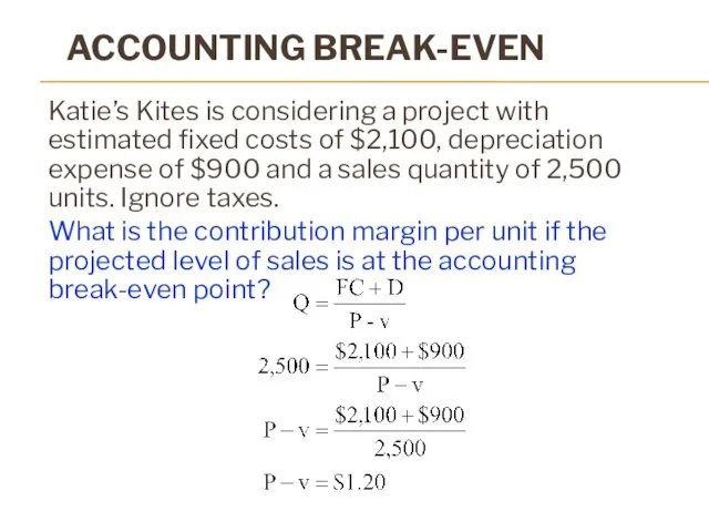
- 20. ACCOUNTING BREAK-EVEN Katie’s Kites is considering a project with estimated fixed costs of $2,100, depreciation expense
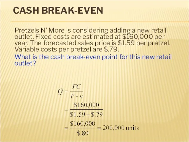
- 21. CASH BREAK-EVEN Pretzels N’ More is considering adding a new retail outlet. Fixed costs are estimated
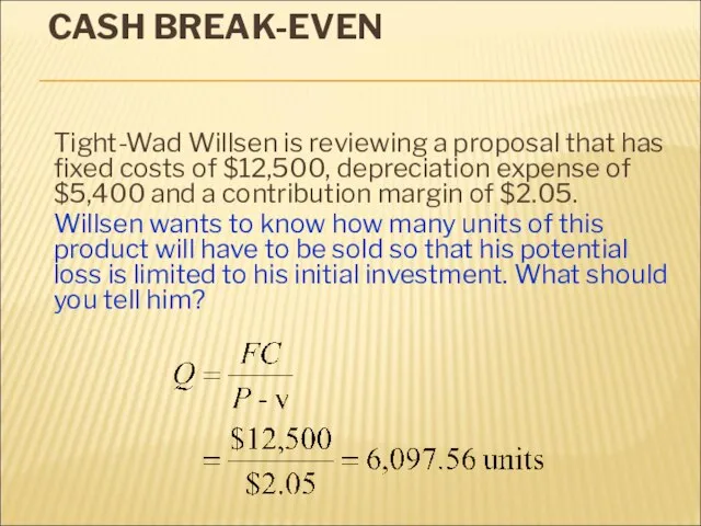
- 22. CASH BREAK-EVEN Tight-Wad Willsen is reviewing a proposal that has fixed costs of $12,500, depreciation expense
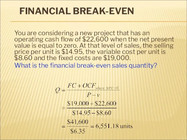
- 23. FINANCIAL BREAK-EVEN You are considering a new project that has an operating cash flow of $22,600
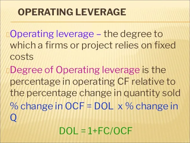
- 24. OPERATING LEVERAGE Operating leverage – the degree to which a firms or project relies on fixed
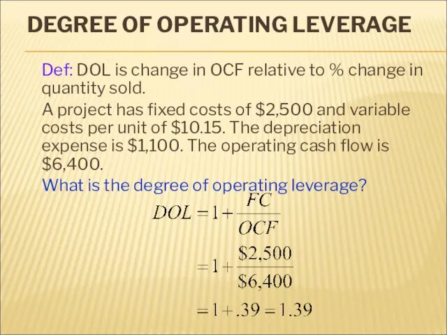
- 25. DEGREE OF OPERATING LEVERAGE Def: DOL is change in OCF relative to % change in quantity
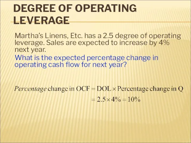
- 26. DEGREE OF OPERATING LEVERAGE Martha’s Linens, Etc. has a 2.5 degree of operating leverage. Sales are
- 28. Скачать презентацию
Слайд 3SCENARIO AND OTHER WHAT-IF ANALYSES
Scenario analysis is the determination of what
SCENARIO AND OTHER WHAT-IF ANALYSES
Scenario analysis is the determination of what
Слайд 4SCENARIO ANALYSIS
Wilson’s Woods is considering a project which involves producing inexpensive golf
SCENARIO ANALYSIS
Wilson’s Woods is considering a project which involves producing inexpensive golf
Слайд 5VARIABLE AND FIXED COSTS
Variable Cost
a cost which is constant per unit but
VARIABLE AND FIXED COSTS
Variable Cost
a cost which is constant per unit but
Слайд 6SCENARIO ANALYSIS
Bob’s Custom Wheels is considering designing and selling customized steering wheels
SCENARIO ANALYSIS
Bob’s Custom Wheels is considering designing and selling customized steering wheels
Слайд 7SENSITIVITY ANALYSIS
Sensitivity analysis is a “what-if” technique that examines how a result
SENSITIVITY ANALYSIS
Sensitivity analysis is a “what-if” technique that examines how a result
Слайд 8SENSITIVITY ANALYSIS
Kettle Corn and Chips is considering selling snack foods at sporting
SENSITIVITY ANALYSIS
Kettle Corn and Chips is considering selling snack foods at sporting
Слайд 9SENSITIVITY ANALYSIS
The Sweet Shoppe is considering opening a kiosk and selling homemade
SENSITIVITY ANALYSIS
The Sweet Shoppe is considering opening a kiosk and selling homemade
Слайд 10SENSITIVITY ANALYSIS
Sales = 6,500 × $1.10 = $7,150
Variable cost = 6,500 × $.69 = $4,485
Fixed cost =
SENSITIVITY ANALYSIS
Sales = 6,500 × $1.10 = $7,150
Variable cost = 6,500 × $.69 = $4,485
Fixed cost =
Слайд 11TOTAL COST
Sandwiches To Go sells 500 sandwiches per day. The company pays
TOTAL COST
Sandwiches To Go sells 500 sandwiches per day. The company pays
Слайд 12AVERAGE VS. MARGINAL COST
Daisy’s Flowers raises and sells 36,000 bouquets of fresh
AVERAGE VS. MARGINAL COST
Daisy’s Flowers raises and sells 36,000 bouquets of fresh
Слайд 13CONTRIBUTION MARGIN
Contribution margin is equal to the difference between total revenue and
CONTRIBUTION MARGIN
Contribution margin is equal to the difference between total revenue and
Слайд 14CONTRIBUTION MARGIN
Jack’s Custom Kars manufactures motorized toy cars for children aged 3
CONTRIBUTION MARGIN
Jack’s Custom Kars manufactures motorized toy cars for children aged 3
Слайд 15COST-VOLUME-PROFIT (BREAKEVEN) GRAPH
$10,000
$8,000
$6,000
$4,000
$2,000
$0
0 10 20 30 40 50
Units Sold
Total
Revenues
Total Costs
Breakeven
Point
25 units
Profits
Losses
COST-VOLUME-PROFIT (BREAKEVEN) GRAPH
$10,000
$8,000
$6,000
$4,000
$2,000
$0
0 10 20 30 40 50
Units Sold
Total
Revenues
Total Costs
Breakeven
Point
25 units
Profits
Losses
Слайд 16BREAKEVEN POINT
Quantity of output where total revenues equal total costs
the point where
BREAKEVEN POINT
Quantity of output where total revenues equal total costs
the point where
Слайд 17BREAKEVEN POINTS
General BE expression – relation between OCF (ignoring taxes) and quantity
BREAKEVEN POINTS
General BE expression – relation between OCF (ignoring taxes) and quantity
Слайд 18BREAKEVEN POINTS
Financial BE – the sales level that results in a zero
BREAKEVEN POINTS
Financial BE – the sales level that results in a zero
Слайд 19ACCOUNTING BREAK-EVEN
You are considering a new project. The projections include a sales
ACCOUNTING BREAK-EVEN
You are considering a new project. The projections include a sales
Слайд 20ACCOUNTING BREAK-EVEN
Katie’s Kites is considering a project with estimated fixed costs of
ACCOUNTING BREAK-EVEN
Katie’s Kites is considering a project with estimated fixed costs of
Слайд 21CASH BREAK-EVEN
Pretzels N’ More is considering adding a new retail outlet. Fixed
CASH BREAK-EVEN
Pretzels N’ More is considering adding a new retail outlet. Fixed
Слайд 22CASH BREAK-EVEN
Tight-Wad Willsen is reviewing a proposal that has fixed costs of
CASH BREAK-EVEN
Tight-Wad Willsen is reviewing a proposal that has fixed costs of
Слайд 23 FINANCIAL BREAK-EVEN
You are considering a new project that has an operating
FINANCIAL BREAK-EVEN
You are considering a new project that has an operating
Слайд 24OPERATING LEVERAGE
Operating leverage – the degree to which a firms or project
OPERATING LEVERAGE
Operating leverage – the degree to which a firms or project
Слайд 25DEGREE OF OPERATING LEVERAGE
Def: DOL is change in OCF relative to %
DEGREE OF OPERATING LEVERAGE
Def: DOL is change in OCF relative to %
Слайд 26DEGREE OF OPERATING LEVERAGE
Martha’s Linens, Etc. has a 2.5 degree of operating
DEGREE OF OPERATING LEVERAGE
Martha’s Linens, Etc. has a 2.5 degree of operating
 Кемеровская Региональная Общественная Организация
 Ароматы для средств по уходу за волосами
 Вебинар для Руководителей Центров Avon
 Сон наяву или приключения в стране чудес
 Цифровое телевидение
 Levels Up Club— это: Прогнозирование финансовых рынков, разработка алгоритмов торговых роботов
 Черты сходства человека и человекообразных обезьян
 Повышение профессиональной компетентности педагогов по вопросам развития речи дошкольников
 Презентация классного коллектива
 Феномен Лапенко
 Энергосберегающие технологии транспорта газа
 Приказ Министерства образования и науки РФ № 209 от 24 марта 2010 г.
 Формы взаимодействия адвоката и следователя на предварительном следствии. Содействие и противодействие
 Поклонюсь Тебя, я, о Боже Нету в целом мире дороже Воспою Тебе хвалу Бог мой я тебя ищу
 РОДИТЕЛЯМ О ПРАВИЛАХ ДОРОЖНОГО ДВИЖЕНИЯ.. Причиной дорожно- транспортных происшествий чаще всего являются сами дети. Приводит к эт
 Конкурс чтецов 1-4 классов в Выльгортской Школе №1
 Дроби
Дроби Презентация по английскому Areas of London Районы Лондона
 Забастовка. Право на забастовку
 ТИПЫ КОСТРОВ
 Продление срока срока службы эпоксидных композитов
 Юлианский Календарь.
 Baroko aktualumas šiais laikais
 Презентация на тему Противоположные числа (6 класс)
 Завтрак чемпиона
 Филиппо Брунеллески
 Презентация1
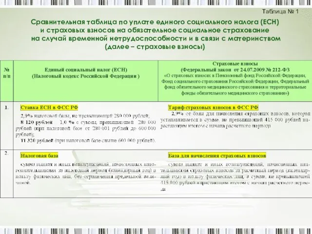 Сравнительная таблица по уплате единого социального налога (ЕСН) и страховых взносов на обязательное социальное страхование на с