- The Aggregate Demand Aggregate Supply

Содержание
- 2. Lecture 3: The Aggregate Demand & Aggregate Supply 1. Aggregate Demand. 2. Aggregate Supply. 3. The
- 3. Lecture 3: The Aggregate Demand & Aggregate Supply Inventory – запаси Overheating – перегрів (економіки)
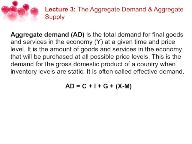
- 4. Lecture 3: The Aggregate Demand & Aggregate Supply Aggregate demand (AD) is the total demand for
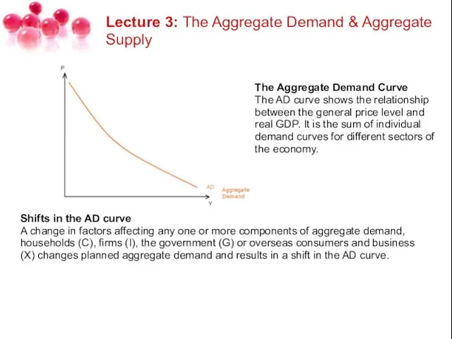
- 5. Lecture 3: The Aggregate Demand & Aggregate Supply The Aggregate Demand Curve The AD curve shows
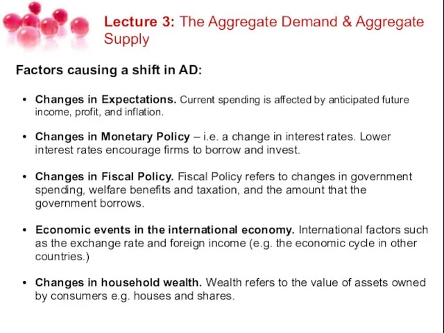
- 6. Lecture 3: The Aggregate Demand & Aggregate Supply Factors causing a shift in AD: Changes in
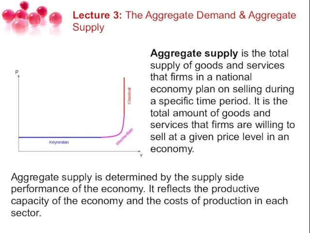
- 7. Lecture 3: The Aggregate Demand & Aggregate Supply Aggregate supply is the total supply of goods
- 8. Lecture 3: The Aggregate Demand & Aggregate Supply There are generally three forms of aggregate supply
- 9. Lecture 3: The Aggregate Demand & Aggregate Supply 2. Long run aggregate supply (LRAS) - Over
- 10. Lecture 3: The Aggregate Demand & Aggregate Supply Shifts in the AS curve can be caused
- 11. Lecture 3: The Aggregate Demand & Aggregate Supply The AD-AS or Aggregate Demand-Aggregate Supply model is
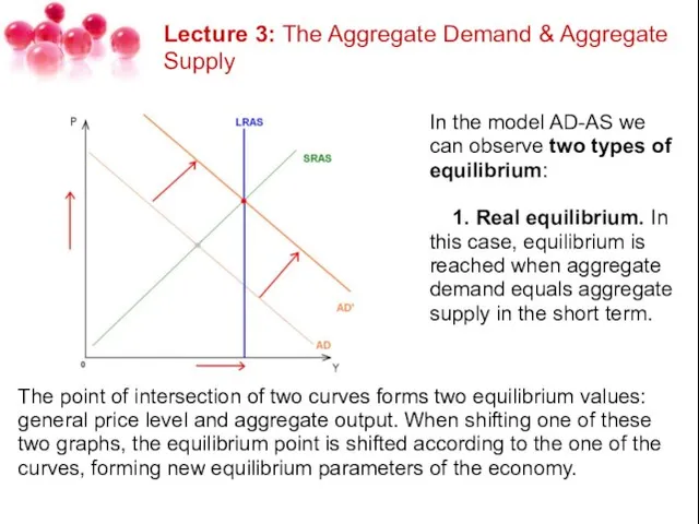
- 12. Lecture 3: The Aggregate Demand & Aggregate Supply In the model AD-AS we can observe two
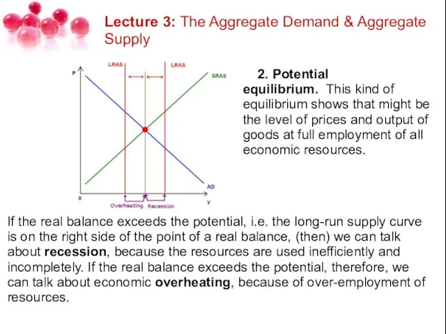
- 13. Lecture 3: The Aggregate Demand & Aggregate Supply 2. Potential equilibrium. This kind of equilibrium shows
- 15. Скачать презентацию
Слайд 2Lecture 3: The Aggregate Demand & Aggregate Supply
1. Aggregate Demand.
2. Aggregate Supply.
3.
Lecture 3: The Aggregate Demand & Aggregate Supply
1. Aggregate Demand.
2. Aggregate Supply.
3.
Слайд 3Lecture 3: The Aggregate Demand & Aggregate Supply
Inventory – запаси
Overheating – перегрів
Lecture 3: The Aggregate Demand & Aggregate Supply
Inventory – запаси
Overheating – перегрів
Слайд 4Lecture 3: The Aggregate Demand & Aggregate Supply
Aggregate demand (AD) is the
Lecture 3: The Aggregate Demand & Aggregate Supply
Aggregate demand (AD) is the
Слайд 5Lecture 3: The Aggregate Demand & Aggregate Supply
The Aggregate Demand Curve
The AD
Lecture 3: The Aggregate Demand & Aggregate Supply
The Aggregate Demand Curve
The AD
Слайд 6Lecture 3: The Aggregate Demand & Aggregate Supply
Factors causing a shift in
Lecture 3: The Aggregate Demand & Aggregate Supply
Factors causing a shift in
Слайд 7Lecture 3: The Aggregate Demand & Aggregate Supply
Aggregate supply is the total
Lecture 3: The Aggregate Demand & Aggregate Supply
Aggregate supply is the total
Слайд 8Lecture 3: The Aggregate Demand & Aggregate Supply
There are generally three forms
Lecture 3: The Aggregate Demand & Aggregate Supply
There are generally three forms
Слайд 9Lecture 3: The Aggregate Demand & Aggregate Supply
2. Long run aggregate
Lecture 3: The Aggregate Demand & Aggregate Supply
2. Long run aggregate
Слайд 10Lecture 3: The Aggregate Demand & Aggregate Supply
Shifts in the AS curve
Lecture 3: The Aggregate Demand & Aggregate Supply
Shifts in the AS curve
Слайд 11Lecture 3: The Aggregate Demand & Aggregate Supply
The AD-AS or Aggregate
Lecture 3: The Aggregate Demand & Aggregate Supply
The AD-AS or Aggregate
Слайд 12Lecture 3: The Aggregate Demand & Aggregate Supply
In the model AD-AS we
Lecture 3: The Aggregate Demand & Aggregate Supply
In the model AD-AS we
Слайд 13Lecture 3: The Aggregate Demand & Aggregate Supply
2. Potential equilibrium. This
Lecture 3: The Aggregate Demand & Aggregate Supply
2. Potential equilibrium. This
 Отчёт о деятельности исполкома TARENA в 2007году и задачи на 2008 год. Руководитель Исполкома TARENA академик МИА и МАНВШ, профессор Садык
 Презентация на тему Проверь свои знания правил пожарной безопасности
 Животный мир степей России
 Шаблон презентации для магистерской диссертации. Луганский национальный университет имени Тараса Шевченко
 Викторина о профессиях
 Песколовки
 Презентация на тему Суд и процесс
  Лекция 7. Городское и сельское население.
 Офисное помещение 181 кв.м на Невском, напротив метро «Маяковская»
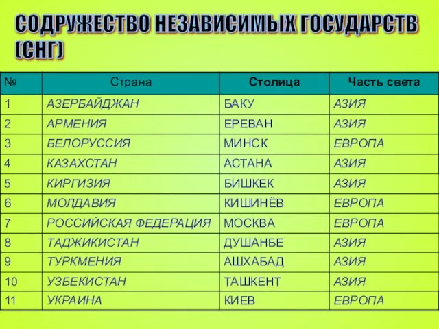 Содружество Независимых Государств (СНГ)
 ФИЗИОЛОГИЧЕСКИЕ ОСНОВЫ АДАПТАЦИИ К ФИЗИЧЕСКИМ НАГРУЗКАМ
 МОНТЁРСКИЙ РЭП
 «Я не писательница, у меня есть профессия…»
 Презентация на тему Социальная мобильность
  Ателье-мастерская
 Подготовка к ЕГЭ по обществознанию
 Методики управления материальными запасами хозяйствующего субъекта
 Моя конвенция
 Техника бега на короткие дистанции
 Обои и шторы
 Презентация Научная и популярная психология для Клуба
 Сборочный чертёж
  ДЕКЛАРИРОВАНИЕ РОЗНИЧНОЙ ПРОДАЖИ АЛКОГОЛЬНОЙ И СПИРТОСОДЕРЖАЩЕЙ ПРОДУКЦИИ
 Класс Земноводные или Амфибии
 Суперкомпьютеры
 в школе
 Научно-производственное предприятие «Грант»
 Открытие магазина DNS в г. Межгорье, требуются универсальные продавцы-консультанты