- Cryogenics & Cryomodules. Part 1: Catching Cold

Содержание
- 2. Goal The goal of this tutorial is to provide a background in cryogenics suitable for workers
- 3. Outline Part 1: Catching Cold Introduction To Cryogenics Basic refrigeration processes Isenthalpic (Joule-Thomson) Isentropic expansion Carnot
- 4. Outline Part 2: Keeping Cold Cryogenic Safety Oxygen Deficiency Hazards Pressure safety High Level Guidelines Cryostats
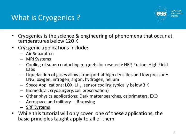
- 5. What is Cryogenics ? Cryogenics is the science & engineering of phenomena that occur at temperatures
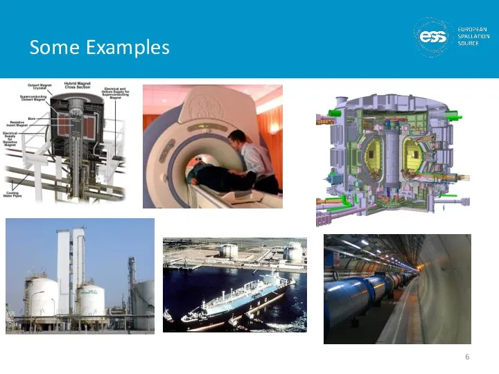
- 6. Some Examples
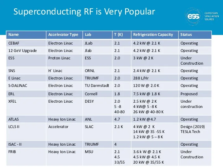
- 7. Superconducting RF is Very Popular
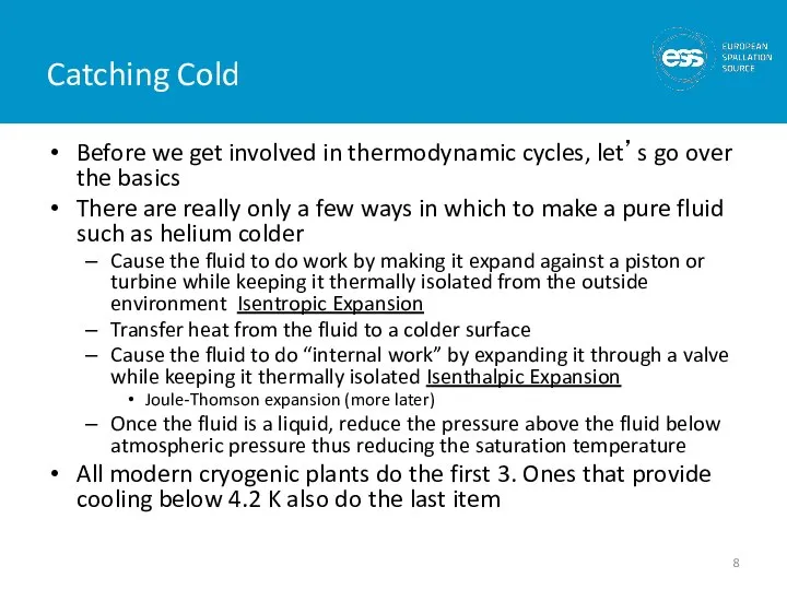
- 8. Catching Cold Before we get involved in thermodynamic cycles, let’s go over the basics There are
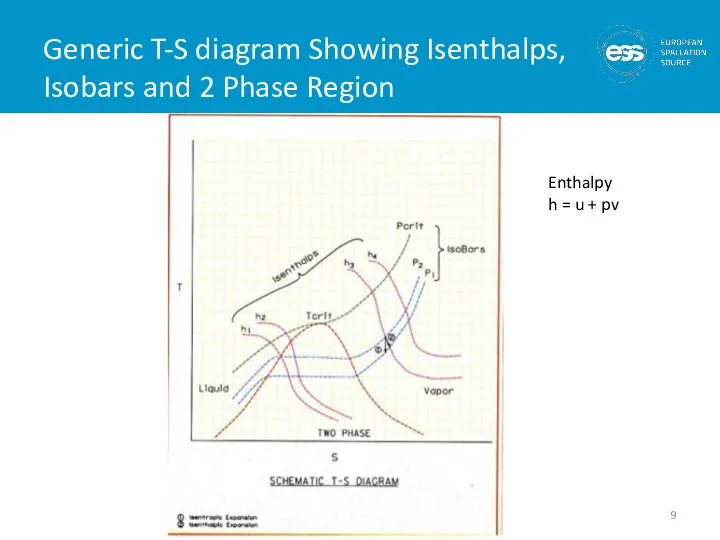
- 9. Generic T-S diagram Showing Isenthalps, Isobars and 2 Phase Region Enthalpy h = u + pv
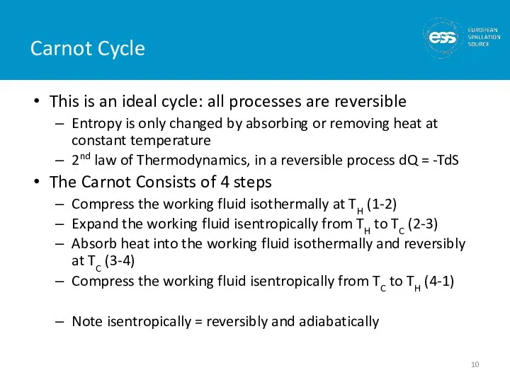
- 10. Carnot Cycle This is an ideal cycle: all processes are reversible Entropy is only changed by
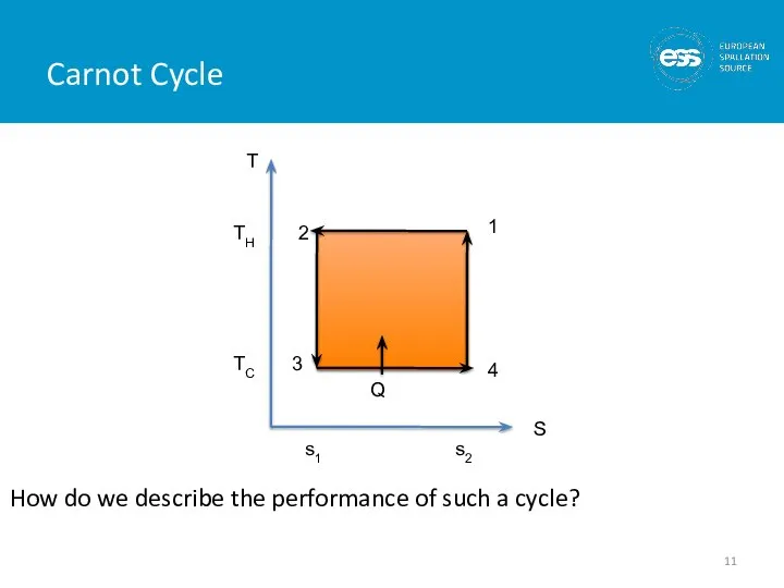
- 11. Carnot Cycle How do we describe the performance of such a cycle?
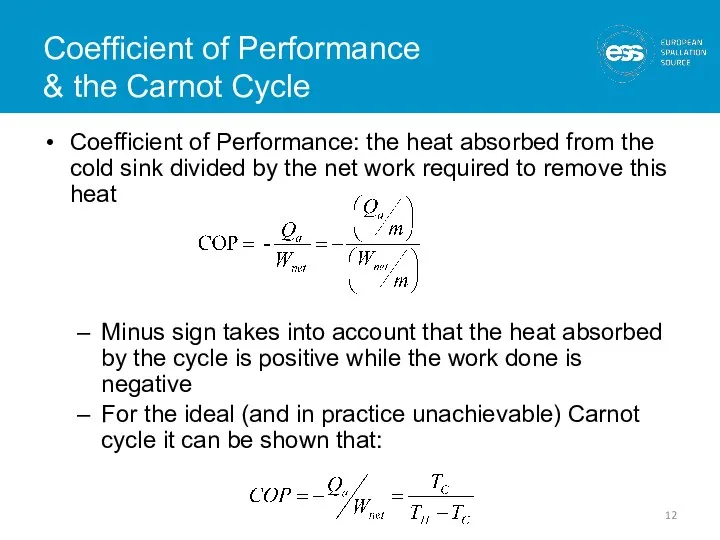
- 12. Coefficient of Performance & the Carnot Cycle Coefficient of Performance: the heat absorbed from the cold
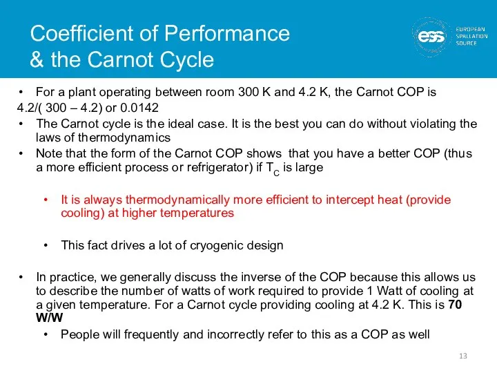
- 13. Coefficient of Performance & the Carnot Cycle For a plant operating between room 300 K and
- 14. Carnot Cycles & the Real World Can we build a real machine using a Carnot cycle?
- 15. The real world is sometimes not kind to cryogenic engineers These are state of the art
- 16. Practical Impact of Plant Performance How much power does it take to operate a large cryogenic
- 17. Joule-Thomson Expansion Isenthalpic (h=constant) expansion Fluid cools as is it is expanded at constant enthalpy through
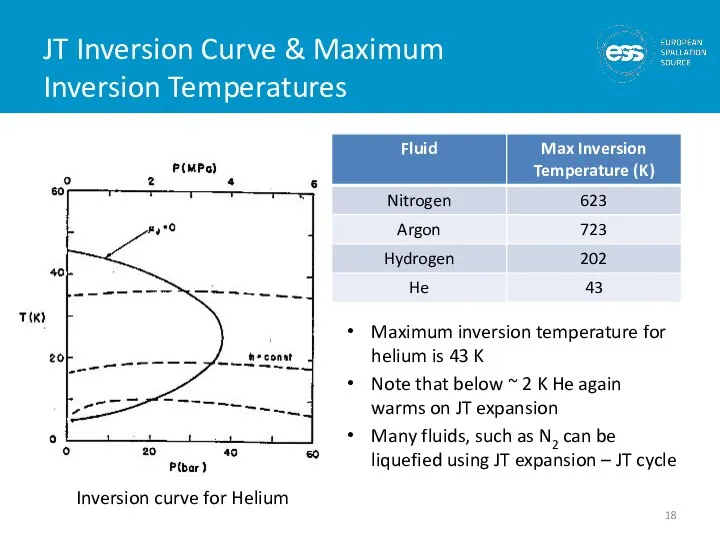
- 18. JT Inversion Curve & Maximum Inversion Temperatures Maximum inversion temperature for helium is 43 K Note
- 19. Practical Large Scale Helium Refrigerators Modern large scale Helium refrigerators/liquefiers use a variation of the Claude
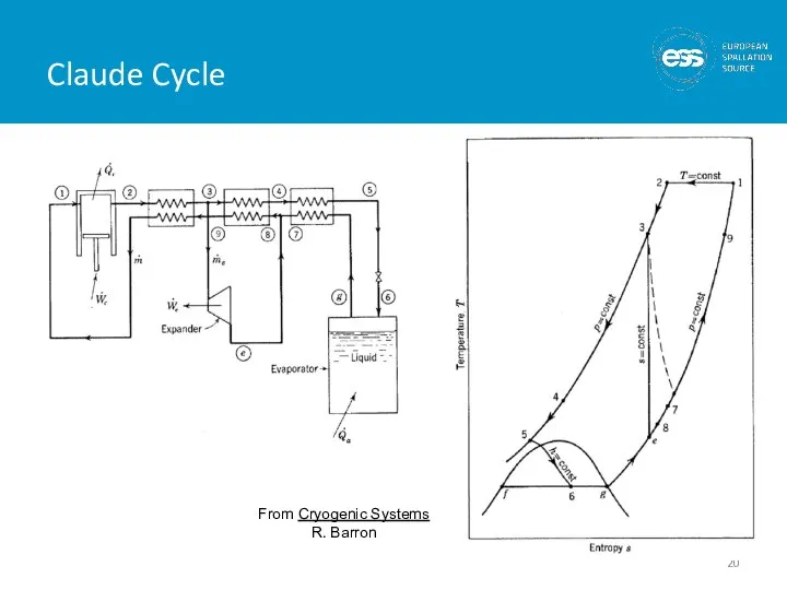
- 20. Claude Cycle From Cryogenic Systems R. Barron
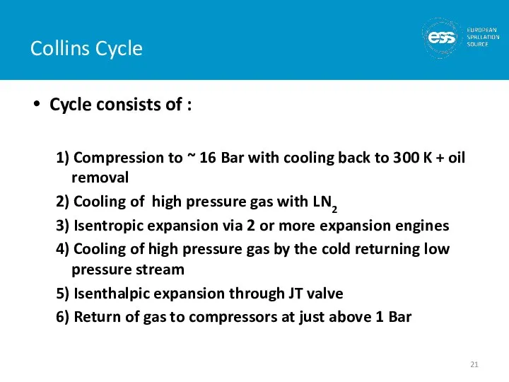
- 21. Cycle consists of : 1) Compression to ~ 16 Bar with cooling back to 300 K
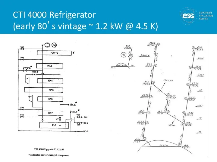
- 22. CTI 4000 Refrigerator (early 80’s vintage ~ 1.2 kW @ 4.5 K)
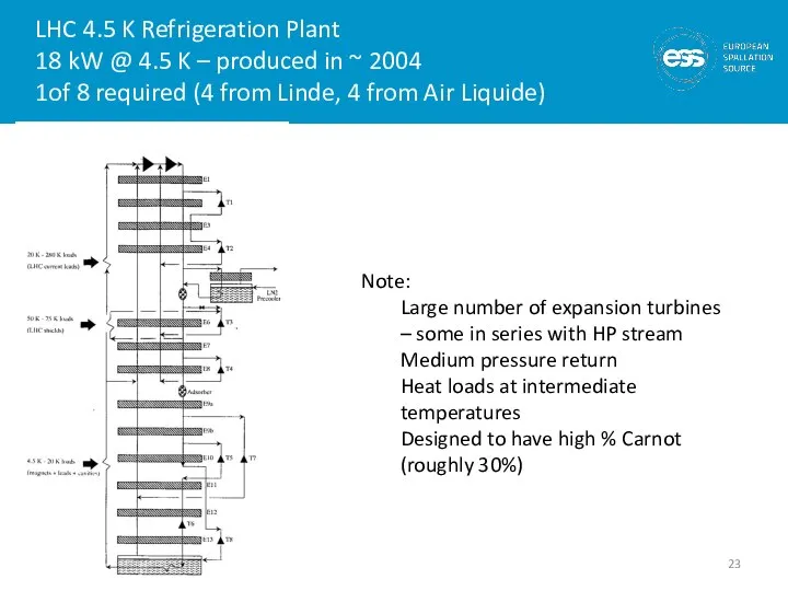
- 23. LHC 4.5 K Refrigeration Plant 18 kW @ 4.5 K – produced in ~ 2004 1of
- 24. Refrigerators vs. Liquefiers Refrigerators are closed cycle systems They provide cooling and can create liquids but
- 25. Refrigerators vs. Liquefiers In practice, this distinction is less clear cut Modern cryogenic plants can operate
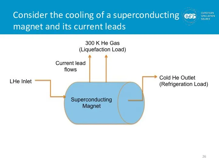
- 26. Consider the cooling of a superconducting magnet and its current leads
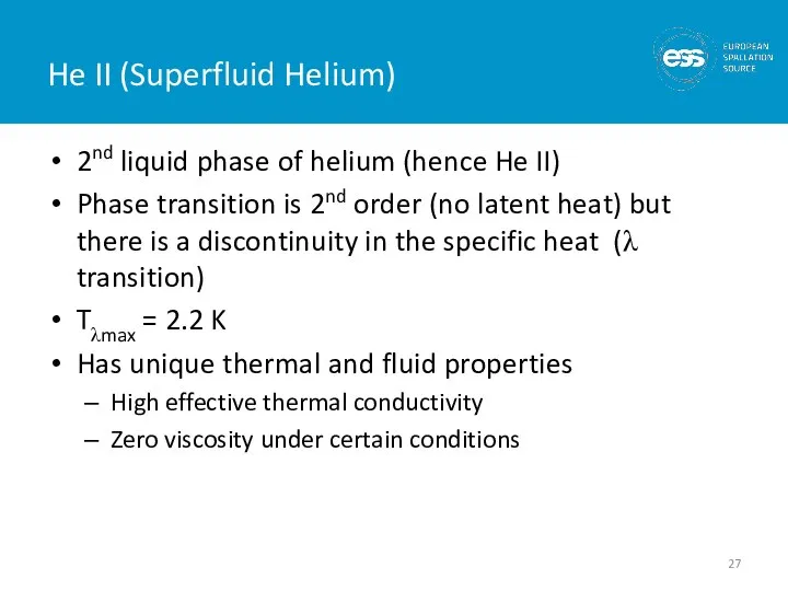
- 27. He II (Superfluid Helium) 2nd liquid phase of helium (hence He II) Phase transition is 2nd
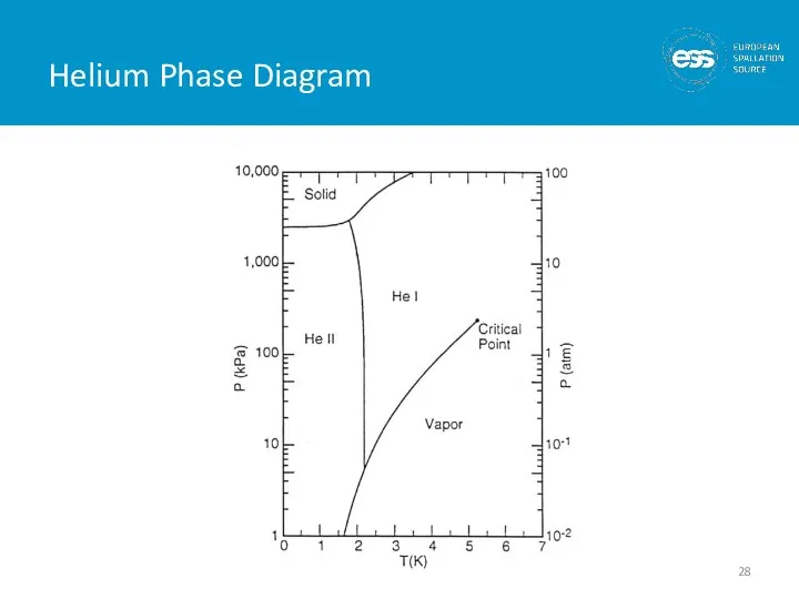
- 28. Helium Phase Diagram
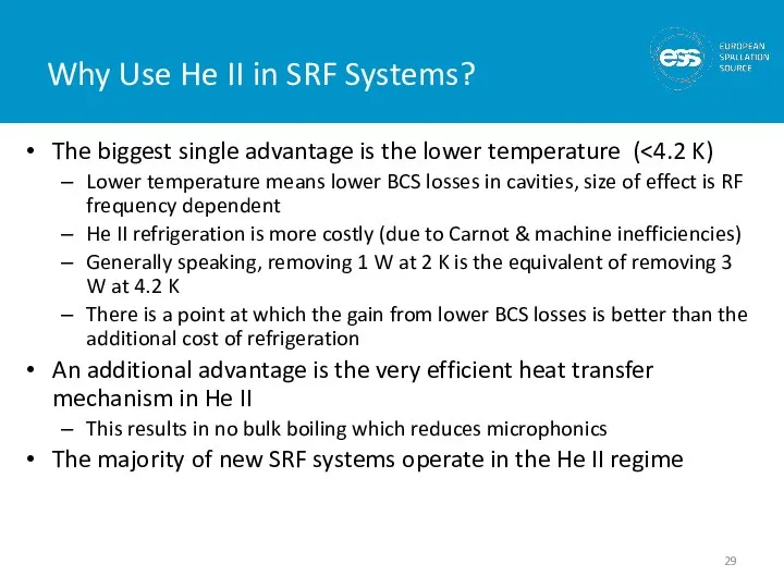
- 29. Why Use He II in SRF Systems? The biggest single advantage is the lower temperature (
- 30. What is He II ? A “Bose – Einstein like” Condensate A fraction of atoms in
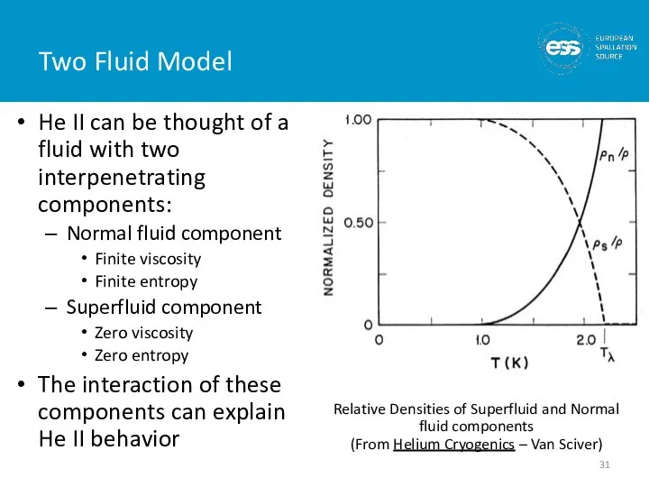
- 31. Two Fluid Model He II can be thought of a fluid with two interpenetrating components: Normal
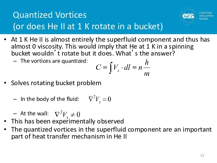
- 32. Quantized Vortices (or does He II at 1 K rotate in a bucket) At 1 K
- 33. Direct Observation of Quantized Vortices via Electron Trapping
- 34. Heat Transfer in He II The basic mechanism is internal convection: No net mass flow Note
- 35. Heat Transfer in He II There are 2 heat transfer regimes: Vs Vs > V sc
- 36. Heat Conductivity Function
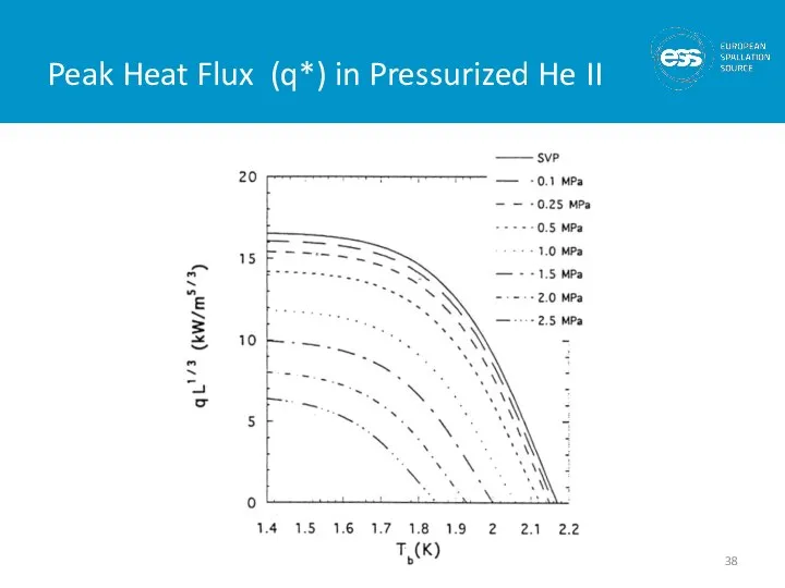
- 37. He II Heat Transfer Limits In pressurized He II: T h must be less than T
- 38. Peak Heat Flux (q*) in Pressurized He II
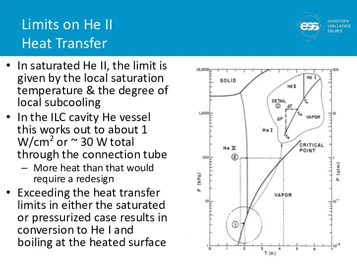
- 39. Limits on He II Heat Transfer In saturated He II, the limit is given by the
- 40. Surface Heat Transfer Heat transfer from a surface into He II is completely dominated by a
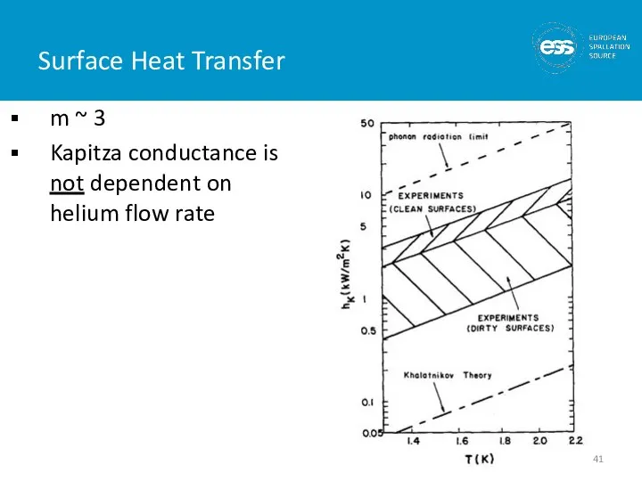
- 41. Surface Heat Transfer m ~ 3 Kapitza conductance is not dependent on helium flow rate
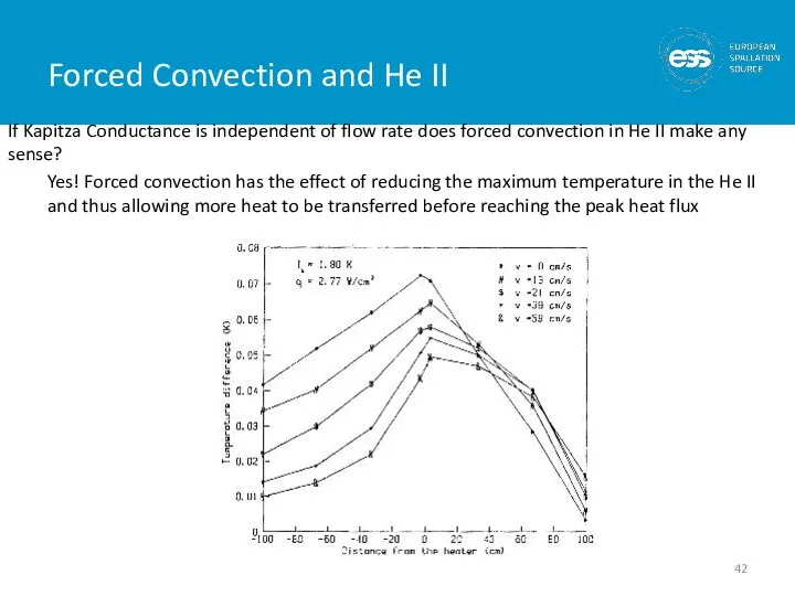
- 42. Forced Convection and He II If Kapitza Conductance is independent of flow rate does forced convection
- 43. He II Fluid Dynamics Despite the presence of the superfluid component, in almost all engineering applications
- 44. He II Fluid Dynamics He II does behave differently in cases of: Film flow Porous plugs
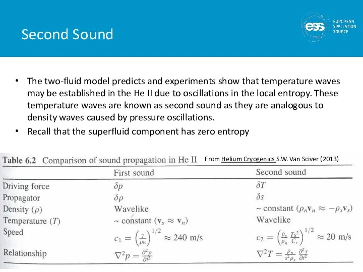
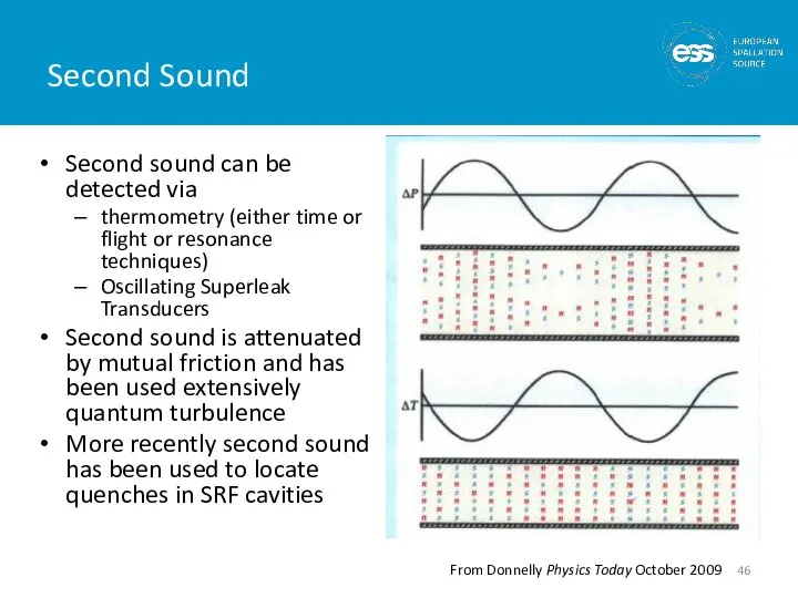
- 45. Second Sound The two-fluid model predicts and experiments show that temperature waves may be established in
- 46. Second Sound Second sound can be detected via thermometry (either time or flight or resonance techniques)
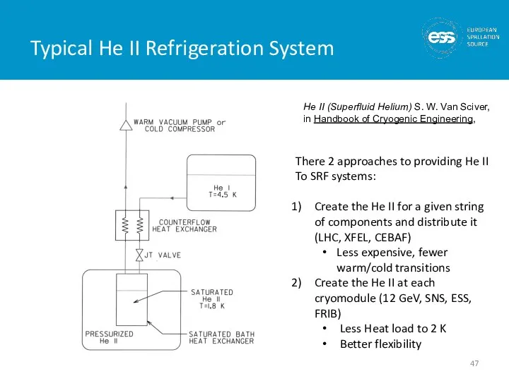
- 47. Typical He II Refrigeration System He II (Superfluid Helium) S. W. Van Sciver, in Handbook of
- 49. Скачать презентацию
Слайд 3Outline
Part 1: Catching Cold
Introduction To Cryogenics
Basic refrigeration processes
Isenthalpic (Joule-Thomson)
Isentropic expansion
Carnot Cycle, COP
Outline
Part 1: Catching Cold
Introduction To Cryogenics
Basic refrigeration processes
Isenthalpic (Joule-Thomson)
Isentropic expansion
Carnot Cycle, COP
Слайд 4Outline
Part 2: Keeping Cold
Cryogenic Safety
Oxygen Deficiency Hazards
Pressure safety
High Level Guidelines
Cryostats and Cryomodules
Definitions
Materials
Thermal
Outline
Part 2: Keeping Cold
Cryogenic Safety
Oxygen Deficiency Hazards
Pressure safety
High Level Guidelines
Cryostats and Cryomodules
Definitions
Materials
Thermal
Слайд 5What is Cryogenics ?
Cryogenics is the science & engineering of phenomena that
What is Cryogenics ?
Cryogenics is the science & engineering of phenomena that
Слайд 6Some Examples
Some Examples
Слайд 7Superconducting RF is Very Popular
Superconducting RF is Very Popular
Слайд 8Catching Cold
Before we get involved in thermodynamic cycles, let’s go over the
Catching Cold
Before we get involved in thermodynamic cycles, let’s go over the
Слайд 9Generic T-S diagram Showing Isenthalps, Isobars and 2 Phase Region
Enthalpy
h = u
Generic T-S diagram Showing Isenthalps, Isobars and 2 Phase Region
Enthalpy
h = u
Слайд 10Carnot Cycle
This is an ideal cycle: all processes are reversible
Entropy is only
Carnot Cycle
This is an ideal cycle: all processes are reversible
Entropy is only
Слайд 11Carnot Cycle
How do we describe the performance of such a cycle?
Carnot Cycle
How do we describe the performance of such a cycle?
Слайд 12Coefficient of Performance
& the Carnot Cycle
Coefficient of Performance: the heat absorbed
Coefficient of Performance
& the Carnot Cycle
Coefficient of Performance: the heat absorbed
Слайд 13Coefficient of Performance
& the Carnot Cycle
For a plant operating between room
Coefficient of Performance
& the Carnot Cycle
For a plant operating between room
Слайд 14Carnot Cycles & the Real World
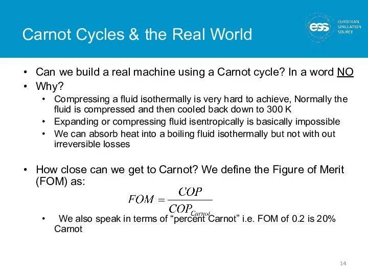
Can we build a real machine using
Carnot Cycles & the Real World
Can we build a real machine using
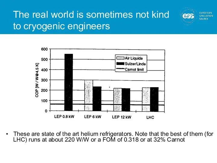
Слайд 15The real world is sometimes not kind to cryogenic engineers
These are state
The real world is sometimes not kind to cryogenic engineers
These are state
Слайд 16Practical Impact of Plant Performance
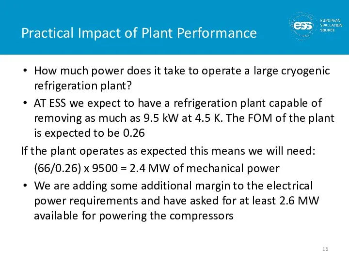
How much power does it take to operate
Practical Impact of Plant Performance
How much power does it take to operate
Слайд 17Joule-Thomson Expansion
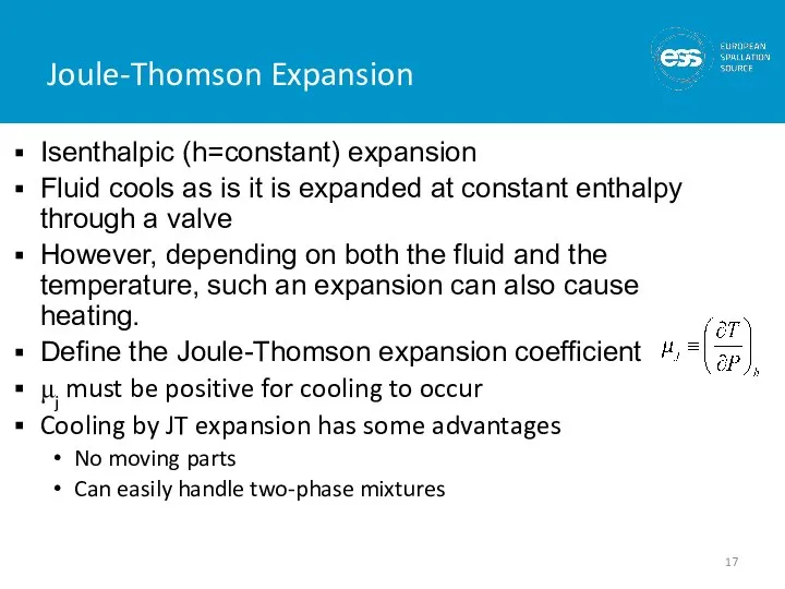
Isenthalpic (h=constant) expansion
Fluid cools as is it is expanded at constant
Joule-Thomson Expansion
Isenthalpic (h=constant) expansion
Fluid cools as is it is expanded at constant
Слайд 18JT Inversion Curve & Maximum
Inversion Temperatures
Maximum inversion temperature for helium is
JT Inversion Curve & Maximum
Inversion Temperatures
Maximum inversion temperature for helium is
Слайд 19Practical Large Scale Helium Refrigerators
Modern large scale Helium refrigerators/liquefiers use a variation
Practical Large Scale Helium Refrigerators
Modern large scale Helium refrigerators/liquefiers use a variation
Слайд 20Claude Cycle
From Cryogenic Systems
R. Barron
Claude Cycle
From Cryogenic Systems
R. Barron
Слайд 21Cycle consists of :
1) Compression to ~ 16 Bar with cooling back
Cycle consists of :
1) Compression to ~ 16 Bar with cooling back
Слайд 22CTI 4000 Refrigerator
(early 80’s vintage ~ 1.2 kW @ 4.5 K)
CTI 4000 Refrigerator
(early 80’s vintage ~ 1.2 kW @ 4.5 K)
Слайд 23LHC 4.5 K Refrigeration Plant
18 kW @ 4.5 K – produced in
LHC 4.5 K Refrigeration Plant 18 kW @ 4.5 K – produced in
Слайд 24Refrigerators vs. Liquefiers
Refrigerators are closed cycle systems
They provide cooling and can create
Refrigerators vs. Liquefiers
Refrigerators are closed cycle systems
They provide cooling and can create
Слайд 25Refrigerators vs. Liquefiers
In practice, this distinction is less clear cut
Modern cryogenic plants
Refrigerators vs. Liquefiers
In practice, this distinction is less clear cut
Modern cryogenic plants
Слайд 26Consider the cooling of a superconducting magnet and its current leads
Consider the cooling of a superconducting magnet and its current leads
Слайд 27He II (Superfluid Helium)
2nd liquid phase of helium (hence He II)
Phase transition
He II (Superfluid Helium)
2nd liquid phase of helium (hence He II)
Phase transition
Слайд 28Helium Phase Diagram
Helium Phase Diagram
Слайд 29Why Use He II in SRF Systems?
The biggest single advantage is the
Why Use He II in SRF Systems?
The biggest single advantage is the
Слайд 30What is He II ?
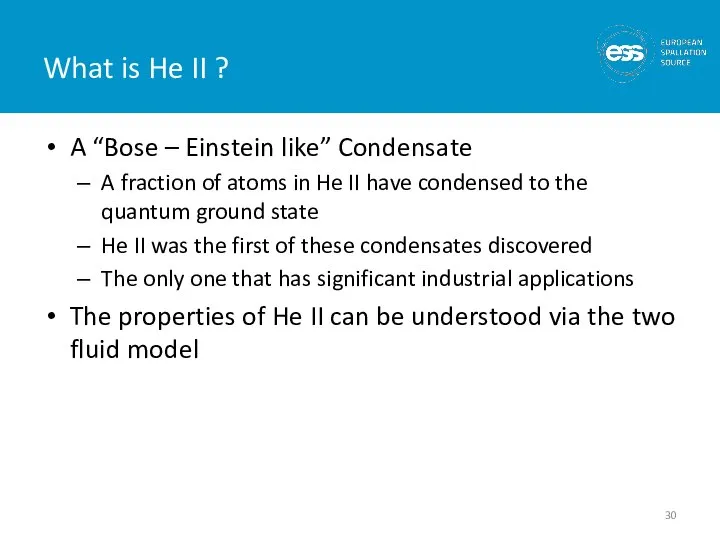
A “Bose – Einstein like” Condensate
A fraction of
What is He II ?
A “Bose – Einstein like” Condensate
A fraction of
Слайд 31Two Fluid Model
He II can be thought of a fluid with two
Two Fluid Model
He II can be thought of a fluid with two
Слайд 32Quantized Vortices
(or does He II at 1 K rotate in a bucket)
At
Quantized Vortices
(or does He II at 1 K rotate in a bucket)
At
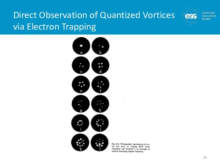
Слайд 33Direct Observation of Quantized Vortices via Electron Trapping
Direct Observation of Quantized Vortices via Electron Trapping
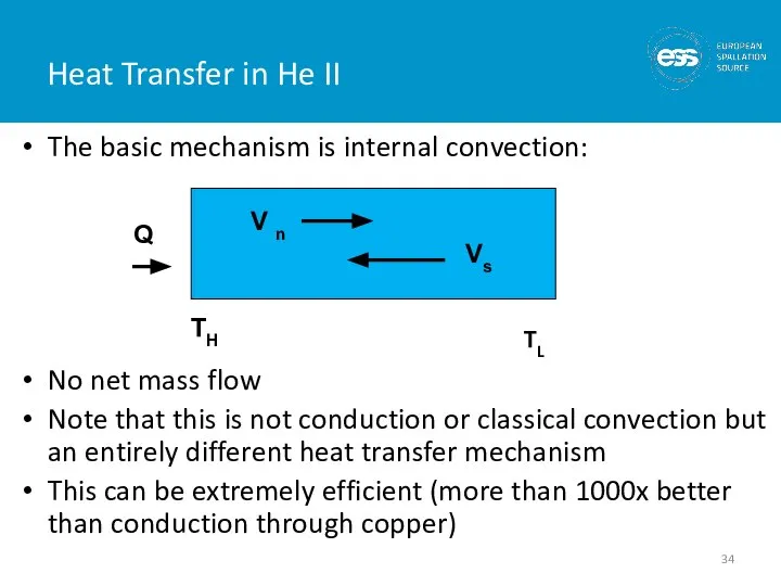
Слайд 34Heat Transfer in He II
The basic mechanism is internal convection:
No net mass
Heat Transfer in He II
The basic mechanism is internal convection:
No net mass
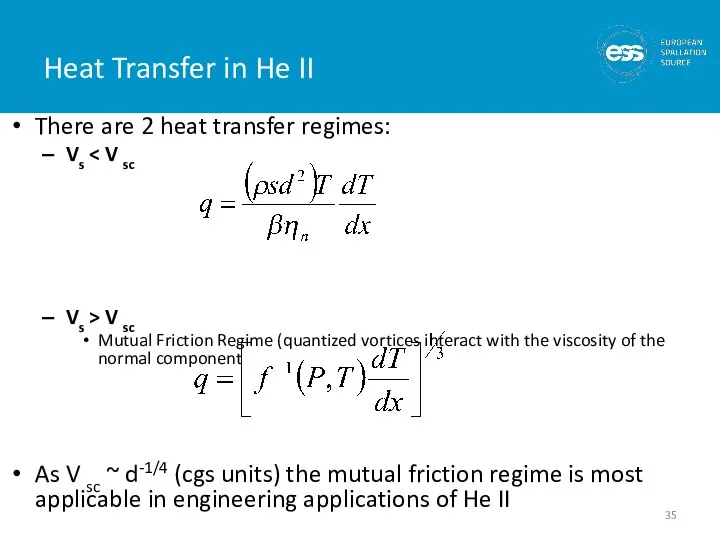
Слайд 35Heat Transfer in He II
There are 2 heat transfer regimes:
Vs < V
Heat Transfer in He II
There are 2 heat transfer regimes:
Vs < V
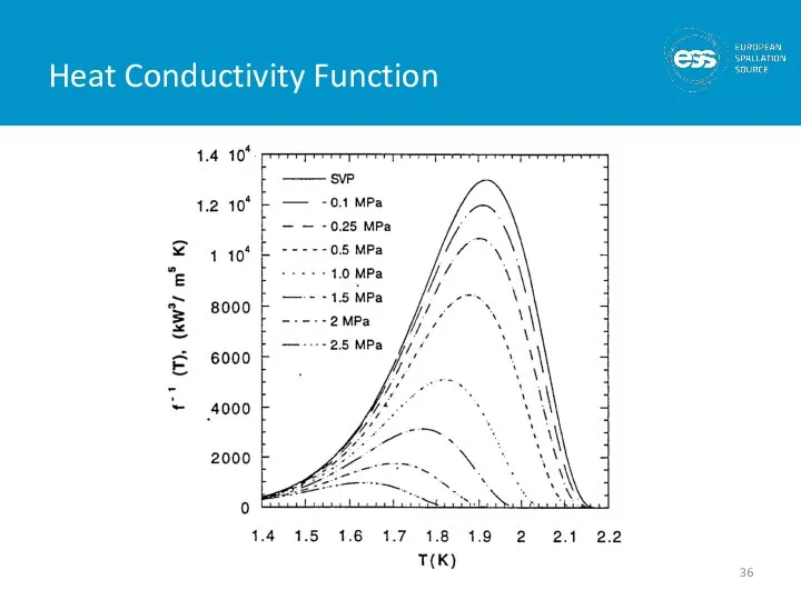
Слайд 36Heat Conductivity Function
Heat Conductivity Function
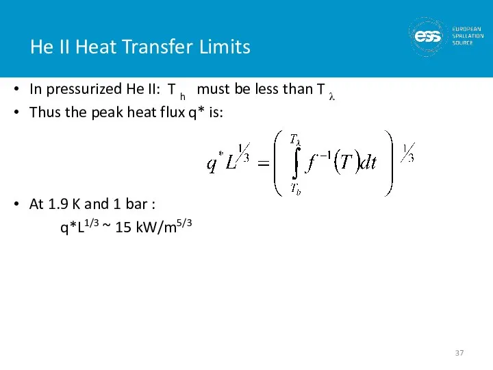
Слайд 37He II Heat Transfer Limits
In pressurized He II: T h must be
He II Heat Transfer Limits
In pressurized He II: T h must be
Слайд 38Peak Heat Flux (q*) in Pressurized He II
Peak Heat Flux (q*) in Pressurized He II
Слайд 39Limits on He II
Heat Transfer
In saturated He II, the limit is
Limits on He II
Heat Transfer
In saturated He II, the limit is
Слайд 40Surface Heat Transfer
Heat transfer from a surface into He II is completely
Surface Heat Transfer
Heat transfer from a surface into He II is completely
Слайд 41Surface Heat Transfer
m ~ 3
Kapitza conductance is not dependent on helium
Surface Heat Transfer
m ~ 3
Kapitza conductance is not dependent on helium
Слайд 42Forced Convection and He II
If Kapitza Conductance is independent of flow rate
Forced Convection and He II
If Kapitza Conductance is independent of flow rate
Слайд 43He II Fluid Dynamics
Despite the presence of the superfluid component, in almost
He II Fluid Dynamics
Despite the presence of the superfluid component, in almost
Слайд 44He II Fluid Dynamics
He II does behave differently in cases of:
Film
He II Fluid Dynamics
He II does behave differently in cases of:
Film
Слайд 45Second Sound
The two-fluid model predicts and experiments show that temperature waves may
Second Sound
The two-fluid model predicts and experiments show that temperature waves may
Слайд 46Second Sound
Second sound can be detected via
thermometry (either time or flight or
Second Sound
Second sound can be detected via
thermometry (either time or flight or
Слайд 47Typical He II Refrigeration System
He II (Superfluid Helium) S. W. Van Sciver,
Typical He II Refrigeration System
He II (Superfluid Helium) S. W. Van Sciver,
 Православный приход храма в честь сошествия святого духа г. Саров
 Презентация на тему СВОБОДА И ОТВЕТСТВЕННОСТЬ ЛИЧНОСТИ
  «ОБЩЕУЧЕБНЫЕ УМЕНИЯ И НАВЫКИ -НЕОБХОДИМОЕ УСЛОВИЕ УСПЕШНОГО ОБУЧЕНИЯ»
 Презентация на тему Карты Проппа
 Презентация на тему Дорожные знаки
 Презентация на тему Угол (2 класс)
  State form
 Презентация на тему Показательная функция, ее свойства и график
 Правила игры в футбол
 Презентация на тему Живой организм и его свойства
 Презентация на тему Гигиена органов пищеварения. Желудочно-кишечные инфекции
  Жестокое отношение к детям в семье
 Как происходили олимпийские игры
 Японская модель устойчивого роста – основа пересмотра ИСО 9004:2000
 Акционное предложение. Носки, гольфы с 03.07.2020 по 01.10.2020
 "Детство под защитой»МОУ СОШ №34г.Красноярск
 Повышаем эффективность e-mail кампаний Наталия Соловьёва UniSender
 _8875ca3baa024c341bab62e3afede7e6_MOD-2_PART-III
 Угадай фильм с Винни-пухом
 Security Gateway Virtual Edition (VE)
 Нравственные уроки семьи – нравственные законы жизни
 Строение головного мозга
 Презентация на тему Растения летом и осенью
  Karl von Frisch
 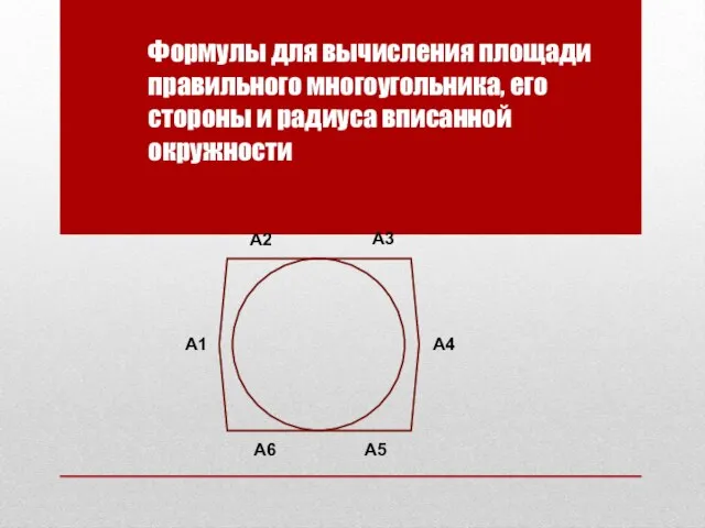 Формулы для площади стороны и радиуса
 Мое хобби
 Менеджер как помощник консультанта по управлению
 Угроза информационной безопасности для детей