- Seismic image regression

Содержание
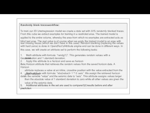
- 2. Randomly blank tracesworkflow: To train our 2D Unetregression model we create a data set with 33%
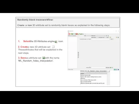
- 3. 1. Selectthe 3D Attributes engine icon. 2. Createa new 3D attribute set Theseattributes that will be
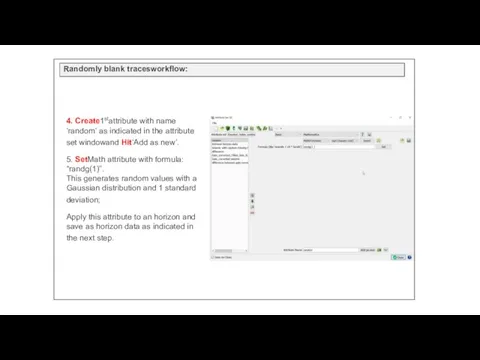
- 4. Randomly blank tracesworkflow: 4. Create1stattribute with name ‘random’ as indicated in the attribute set windowand Hit‘Add
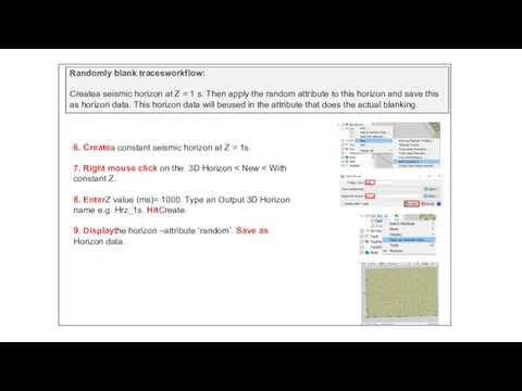
- 5. 6. Createa constant seismic horizon at Z = 1s. 7. Right mouse click on the 3D
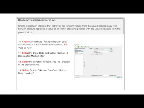
- 6. Randomly blank tracesworkflow: Create an horizon attribute that retrieves the random values from the saved horizon
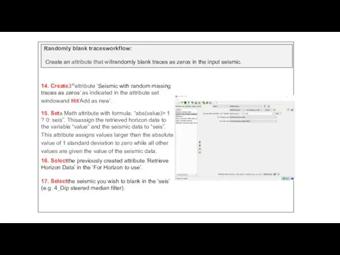
- 7. Randomly blank tracesworkflow: Create an attribute that willrandomly blank traces as zeros in the input seismic.
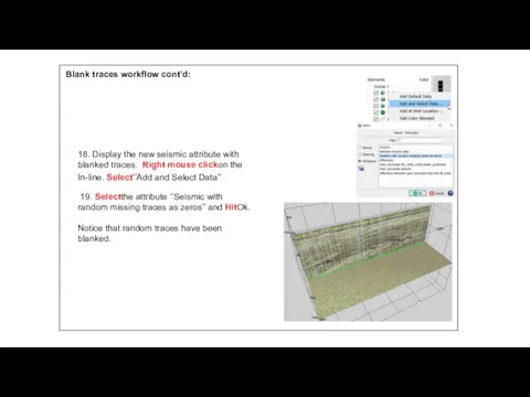
- 8. Blank traces workflow cont’d: 18. Display the new seismic attribute with blanked traces. Right mouse clickon
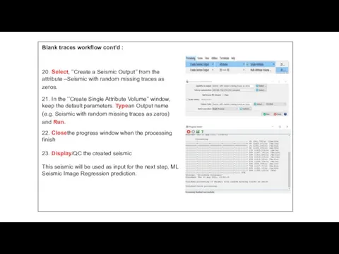
- 9. Blank traces workflow cont’d : 20. Select, ‘’Create a Seismic Output’’ from the attribute –Seismic with
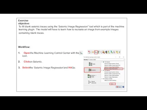
- 10. Exercise objective: To fill blank seismic traces using the ‘Seismic Image Regression’’ tool which is part
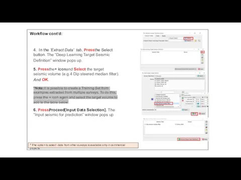
- 11. Workflow cont’d: 4. In the ‘Extract Data’ tab, Pressthe Select button. The “Deep Learning Target Seismic
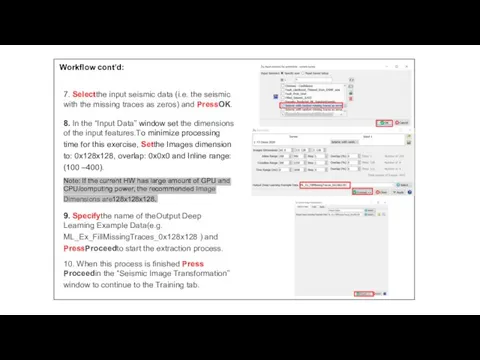
- 12. Workflow cont’d: 7. Selectthe input seismic data (i.e. the seismic with the missing traces as zeros)
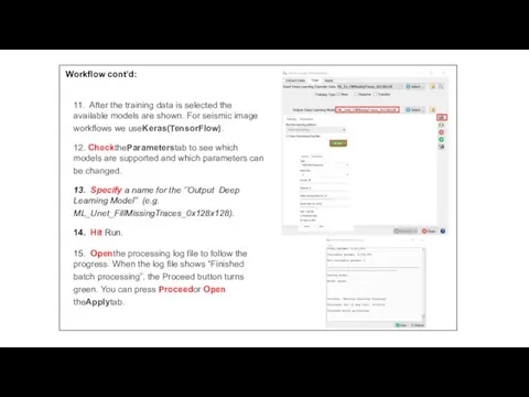
- 13. Workflow cont’d: 11. After the training data is selected the available models are shown. For seismic
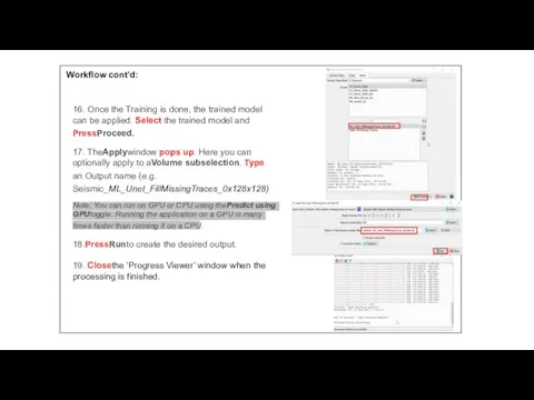
- 14. Workflow cont’d: 16. Once the Training is done, the trained model can be applied. Select the
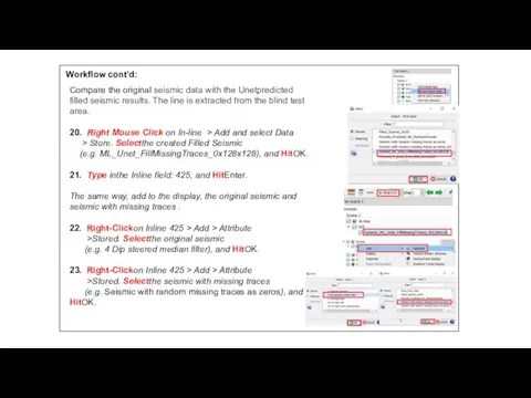
- 15. Workflow cont’d: Compare the original seismic data with the Unetpredicted filled seismic results. The line is
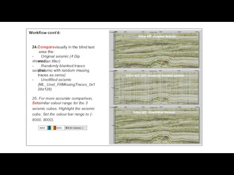
- 16. 24.Comparevisually in the blind test area the: - Original seismic (4 Dip steered median filter) -
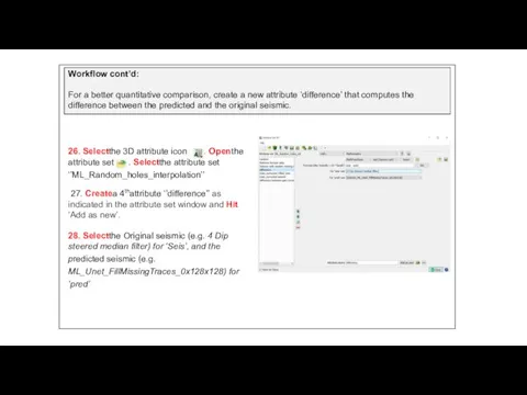
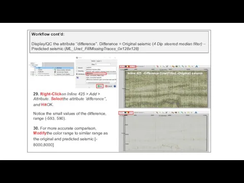
- 17. Workflow cont’d: For a better quantitative comparison, create a new attribute ‘difference’ that computes the difference
- 18. 29. Right-Clickon Inline 425 > Add > Attribute. Selectthe attribute ‘difference’’, and HitOK. Notice the small
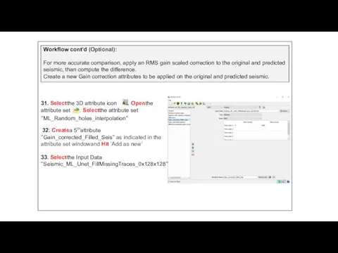
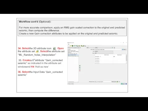
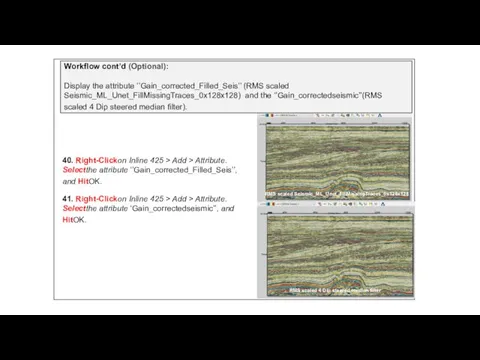
- 19. Workflow cont’d (Optional): For more accurate comparison, apply an RMS gain scaled correction to the original
- 20. 34. Selectthe 3D attribute icon . Open the attribute set . Selectthe attribute set ‘’ML_Random_holes_interpolation’’ 35.
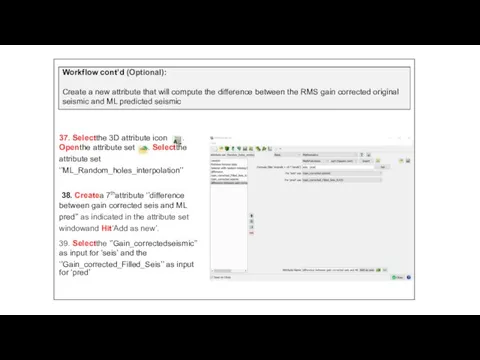
- 21. Workflow cont’d (Optional): Create a new attribute that will compute the difference between the RMS gain
- 22. 40. Right-Clickon Inline 425 > Add > Attribute. Selectthe attribute ‘’Gain_corrected_Filled_Seis’’, and HitOK. 41. Right-Clickon Inline
- 24. Скачать презентацию
Слайд 31. Selectthe 3D Attributes engine icon.
2. Createa new 3D attribute set
Theseattributes
1. Selectthe 3D Attributes engine icon.
2. Createa new 3D attribute set
Theseattributes
Слайд 4Randomly blank tracesworkflow:
4. Create1stattribute with name
‘random’ as indicated in the attribute
Randomly blank tracesworkflow:
4. Create1stattribute with name
‘random’ as indicated in the attribute
Слайд 56. Createa constant seismic horizon at Z = 1s.
7. Right mouse
6. Createa constant seismic horizon at Z = 1s.
7. Right mouse
Слайд 6Randomly blank tracesworkflow:
Create an horizon attribute that retrieves the random values from
Randomly blank tracesworkflow:
Create an horizon attribute that retrieves the random values from
Слайд 7Randomly blank tracesworkflow:
Create an attribute that willrandomly blank traces as zeros in
Randomly blank tracesworkflow:
Create an attribute that willrandomly blank traces as zeros in
Слайд 8Blank traces workflow cont’d:
18. Display the new seismic attribute with
blanked traces.
Blank traces workflow cont’d:
18. Display the new seismic attribute with
blanked traces.
Слайд 9Blank traces workflow cont’d :
20. Select, ‘’Create a Seismic Output’’ from the
Blank traces workflow cont’d :
20. Select, ‘’Create a Seismic Output’’ from the
Слайд 10Exercise objective:
To fill blank seismic traces using the ‘Seismic Image Regression’’ tool
Exercise objective:
To fill blank seismic traces using the ‘Seismic Image Regression’’ tool
Слайд 11Workflow cont’d:
4. In the ‘Extract Data’ tab, Pressthe Select
button. The “Deep
Workflow cont’d:
4. In the ‘Extract Data’ tab, Pressthe Select
button. The “Deep
Слайд 12Workflow cont’d:
7. Selectthe input seismic data (i.e. the seismic
with the missing
Workflow cont’d:
7. Selectthe input seismic data (i.e. the seismic
with the missing
Слайд 13Workflow cont’d:
11. After the training data is selected the
available models are
Workflow cont’d:
11. After the training data is selected the
available models are
Слайд 14Workflow cont’d:
16. Once the Training is done, the trained model
can be
Workflow cont’d:
16. Once the Training is done, the trained model
can be
Слайд 15Workflow cont’d:
Compare the original seismic data with the Unetpredicted
filled seismic results. The
Workflow cont’d:
Compare the original seismic data with the Unetpredicted
filled seismic results. The
Слайд 1624.Comparevisually in the blind test
area the:
- Original seismic (4 Dip steered
median
24.Comparevisually in the blind test
area the:
- Original seismic (4 Dip steered
median
Слайд 17Workflow cont’d:
For a better quantitative comparison, create a new attribute ‘difference’ that
Workflow cont’d:
For a better quantitative comparison, create a new attribute ‘difference’ that
Слайд 1829. Right-Clickon Inline 425 > Add >
Attribute. Selectthe attribute ‘difference’’,
and
29. Right-Clickon Inline 425 > Add >
Attribute. Selectthe attribute ‘difference’’,
and
Слайд 19Workflow cont’d (Optional):
For more accurate comparison, apply an RMS gain scaled correction
Workflow cont’d (Optional):
For more accurate comparison, apply an RMS gain scaled correction
Слайд 2034. Selectthe 3D attribute icon . Open
the attribute set . Selectthe attribute
34. Selectthe 3D attribute icon . Open
the attribute set . Selectthe attribute
Слайд 21Workflow cont’d (Optional):
Create a new attribute that will compute the difference between
Workflow cont’d (Optional):
Create a new attribute that will compute the difference between
Слайд 2240. Right-Clickon Inline 425 > Add > Attribute.
Selectthe attribute ‘’Gain_corrected_Filled_Seis’’,
and
40. Right-Clickon Inline 425 > Add > Attribute.
Selectthe attribute ‘’Gain_corrected_Filled_Seis’’,
and
 Дизайн сайта. Вебинар 2
 Двумерные массивы: работа с диагоналями
 Продвижение библиотеки в социальных сетях. Всероссийский конкурс
 Истинные и ложные утверждения
 Использование встроенного задачника в Pascal ABC
 Создание компьютерных игр
 Программа для выделение движущихся объектов. Лабораторная работа № 2
 Создание графических изображений
 IFS Applications • Компонентная ERP-система • Поддержка 22 языков • Доступна для работы с планшетов и смартфонов
 Прикладне програмування
 Администрирование объектов доступа
 Проблемы современного цифрового общества
 Жанровый состав
 Повышение надёжности функционирования корпоративной телекоммуникационной сети
 Виды и форматы электронных изданий
 Лайфхаки персональной информационной безопасности
 Соционика. Введение
 Робота з Visual Basic в MS Excel 2007
 История интеренета
 Виды алгоритмов. 5 класс
 Скины 187-го легиона
 Разработка веб-приложения для сбора мнений о мероприятиях МКУК
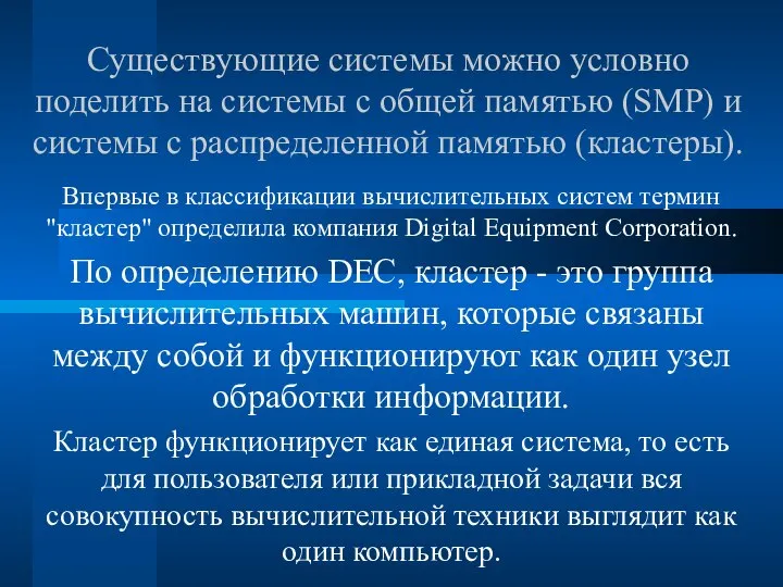 Области применения вычислительных систем (шкала условная, логарифмическая)
 Методика решения олимпиадных задач
 2D графика
 Кодирование чисел в компьютере
 Імітаційне моделювання роботизованої виробничої ділянки
 Цифровой участок для мобильного избирателя. КРОК