- Demand and Aggregate Supply

Содержание
- 2. 10 AGGREGATE SUPPLY AND AGGREGATE DEMAND
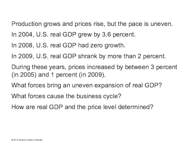
- 4. Production grows and prices rise, but the pace is uneven. In 2004, U.S. real GDP grew
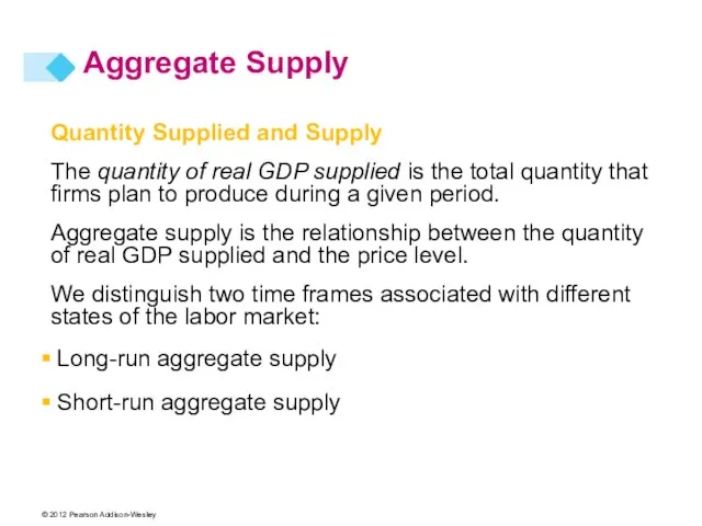
- 5. Quantity Supplied and Supply The quantity of real GDP supplied is the total quantity that firms
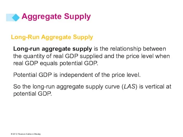
- 6. Long-Run Aggregate Supply Long-run aggregate supply is the relationship between the quantity of real GDP supplied
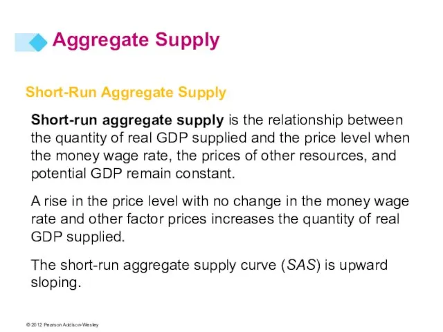
- 7. Short-Run Aggregate Supply Short-run aggregate supply is the relationship between the quantity of real GDP supplied
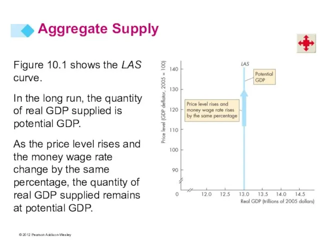
- 8. Figure 10.1 shows the LAS curve. In the long run, the quantity of real GDP supplied
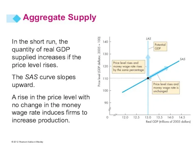
- 9. In the short run, the quantity of real GDP supplied increases if the price level rises.
- 10. With a given money wage rate, the SAS curve cuts the LAS curve at potential GDP.
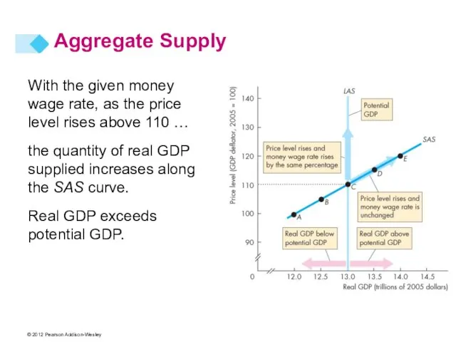
- 11. With the given money wage rate, as the price level rises above 110 … the quantity
- 12. Changes in Aggregate Supply Aggregate supply changes if an influence on production plans other than the
- 13. Changes in Potential GDP When potential GDP increases, both the LAS and SAS curves shift rightward.
- 14. Figure 10.2 shows the effect of an increase in potential GDP. The LAS curve shifts rightward
- 15. Changes in the Money Wage Rate Figure 10.3 shows the effect of a rise in the
- 16. The quantity of real GDP demanded, Y, is the total amount of final goods and services
- 17. Buying plans depend on many factors and some of the main ones are The price level
- 18. Aggregate Demand The Aggregate Demand Curve Aggregate demand is the relationship between the quantity of real
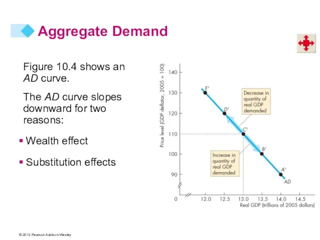
- 19. Figure 10.4 shows an AD curve. The AD curve slopes downward for two reasons: Wealth effect
- 20. Aggregate Demand Wealth Effect A rise in the price level, other things remaining the same, decreases
- 21. Aggregate Demand Substitution Effects Intertemporal substitution effect: A rise in the price level, other things remaining
- 22. Aggregate Demand International substitution effect: A rise in the price level, other things remaining the same,
- 23. Aggregate Demand Changes in Aggregate Demand A change in any influence on buying plans other than
- 24. Aggregate Demand Expectations Expectations about future income, future inflation, and future profits change aggregate demand. Increases
- 25. Aggregate Demand Fiscal Policy and Monetary Policy Fiscal policy is the government’s attempt to influence the
- 26. Aggregate Demand Fiscal Policy and Monetary Policy Because government expenditure on goods and services is one
- 27. Aggregate Demand The World Economy The world economy influences aggregate demand in two ways: A fall
- 28. Aggregate Demand Figure 10.5 illustrates changes in aggregate demand. When aggregate demand increases, the AD curve
- 29. Explaining Macroeconomic Trends and Fluctuations Short-Run Macroeconomic Equilibrium Short-run macroeconomic equilibrium occurs when the quantity of
- 30. Figure 10.6 illustrates a short-run equilibrium. If real GDP is below equilibrium GDP, firms increase production
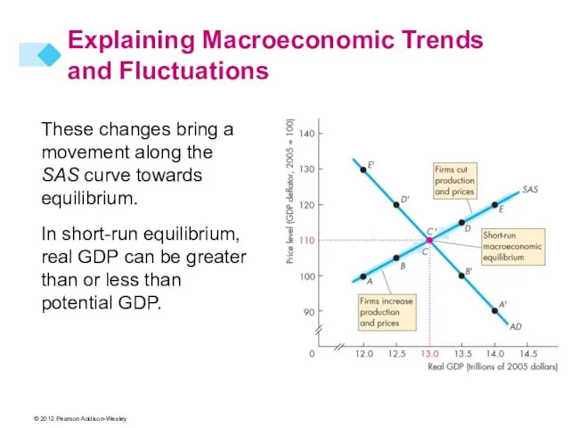
- 31. These changes bring a movement along the SAS curve towards equilibrium. In short-run equilibrium, real GDP
- 32. Long-Run Macroeconomic Equilibrium Long-run macroeconomic equilibrium occurs when real GDP equals potential GDP—when the economy is
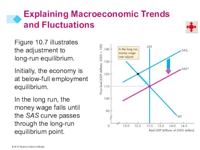
- 33. Figure 10.7 illustrates the adjustment to long-run equilibrium. Initially, the economy is at below-full employment equilibrium.
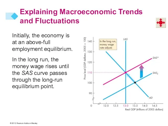
- 34. Initially, the economy is at an above-full employment equilibrium. In the long run, the money wage
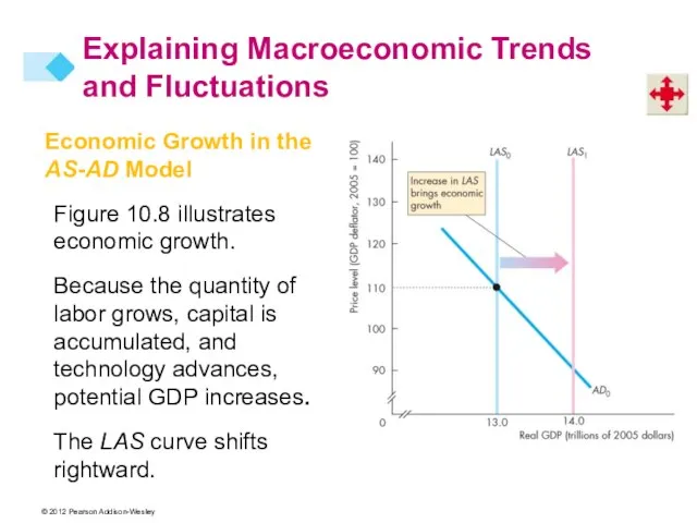
- 35. Economic Growth in the AS-AD Model Figure 10.8 illustrates economic growth. Because the quantity of labor
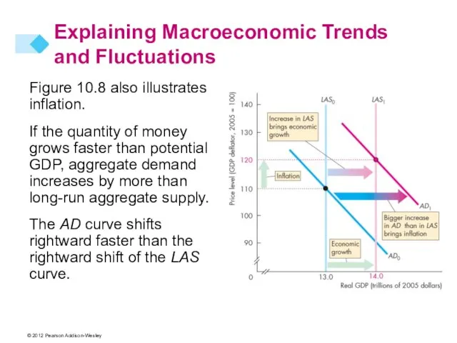
- 36. Figure 10.8 also illustrates inflation. If the quantity of money grows faster than potential GDP, aggregate
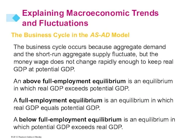
- 37. The Business Cycle in the AS-AD Model The business cycle occurs because aggregate demand and the
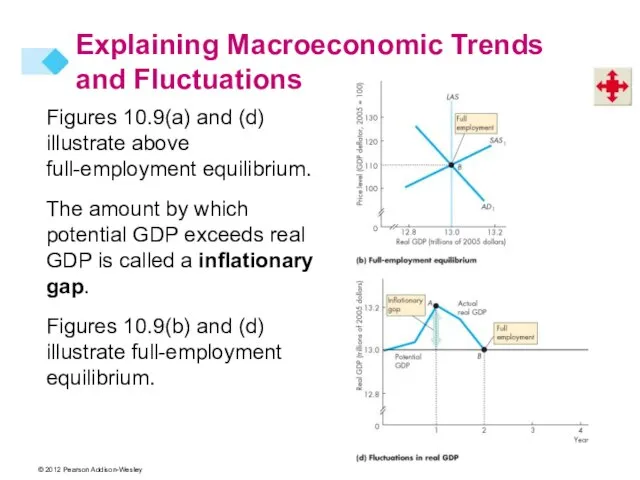
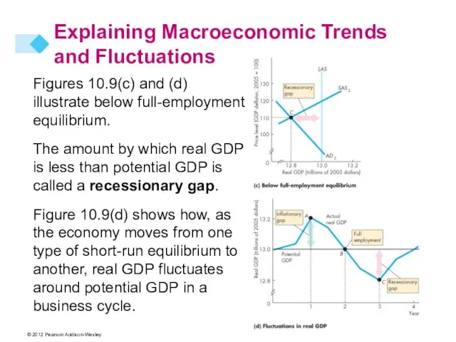
- 38. Figures 10.9(a) and (d) illustrate above full-employment equilibrium. The amount by which potential GDP exceeds real
- 39. Figures 10.9(c) and (d) illustrate below full-employment equilibrium. The amount by which real GDP is less
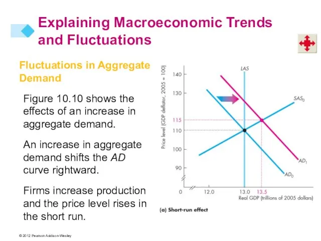
- 40. Fluctuations in Aggregate Demand Figure 10.10 shows the effects of an increase in aggregate demand. An
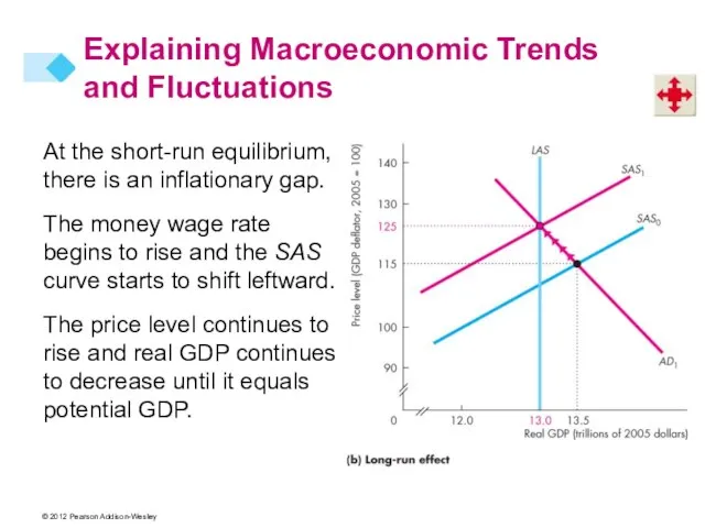
- 41. At the short-run equilibrium, there is an inflationary gap. The money wage rate begins to rise
- 42. Fluctuations in Aggregate Supply Figure 10.11 shows the effects of a rise in the price of
- 43. Macroeconomic Schools of Thought Macroeconomists can be divided into three broad schools of thought: Classical Keynesian
- 44. Macroeconomic Schools of Thought The Classical View A classical macroeconomist believes that the economy is self-regulating
- 45. Macroeconomic Schools of Thought The Keynesian View A Keynesian macroeconomist believes that left alone, the economy
- 47. Скачать презентацию

Слайд 4Production grows and prices rise, but the pace is uneven.
In 2004, U.S.
Production grows and prices rise, but the pace is uneven.
In 2004, U.S.
Слайд 5Quantity Supplied and Supply
The quantity of real GDP supplied is the total
Quantity Supplied and Supply
The quantity of real GDP supplied is the total
Слайд 6Long-Run Aggregate Supply
Long-run aggregate supply is the relationship between the quantity of
Long-Run Aggregate Supply
Long-run aggregate supply is the relationship between the quantity of
Слайд 7Short-Run Aggregate Supply
Short-run aggregate supply is the relationship between the quantity of
Short-Run Aggregate Supply
Short-run aggregate supply is the relationship between the quantity of
Слайд 8Figure 10.1 shows the LAS curve.
In the long run, the quantity of
Figure 10.1 shows the LAS curve.
In the long run, the quantity of
Слайд 9In the short run, the quantity of real GDP supplied increases if
In the short run, the quantity of real GDP supplied increases if
Слайд 10With a given money wage rate, the SAS curve cuts the LAS
With a given money wage rate, the SAS curve cuts the LAS
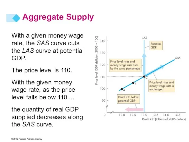
Слайд 11With the given money wage rate, as the price level rises above
With the given money wage rate, as the price level rises above
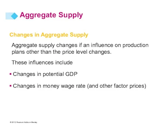
Слайд 12Changes in Aggregate Supply
Aggregate supply changes if an influence on production plans
Changes in Aggregate Supply
Aggregate supply changes if an influence on production plans
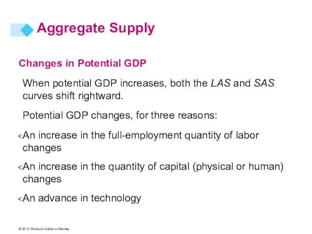
Слайд 13Changes in Potential GDP
When potential GDP increases, both the LAS and SAS
Changes in Potential GDP
When potential GDP increases, both the LAS and SAS
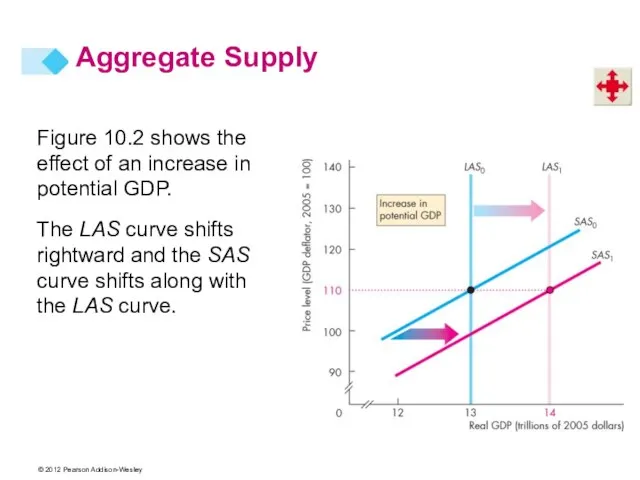
Слайд 14Figure 10.2 shows the effect of an increase in potential GDP.
The LAS
Figure 10.2 shows the effect of an increase in potential GDP.
The LAS
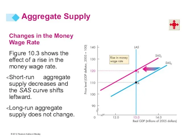
Слайд 15Changes in the Money Wage Rate
Figure 10.3 shows the effect of
Changes in the Money Wage Rate
Figure 10.3 shows the effect of
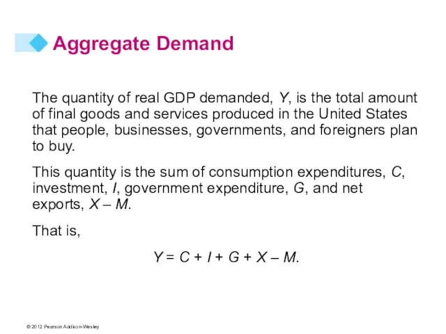
Слайд 16The quantity of real GDP demanded, Y, is the total amount of
The quantity of real GDP demanded, Y, is the total amount of
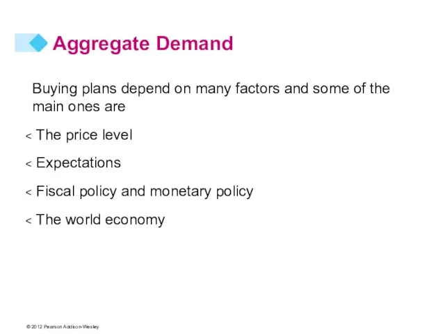
Слайд 17Buying plans depend on many factors and some of the main ones
Buying plans depend on many factors and some of the main ones
Слайд 18Aggregate Demand
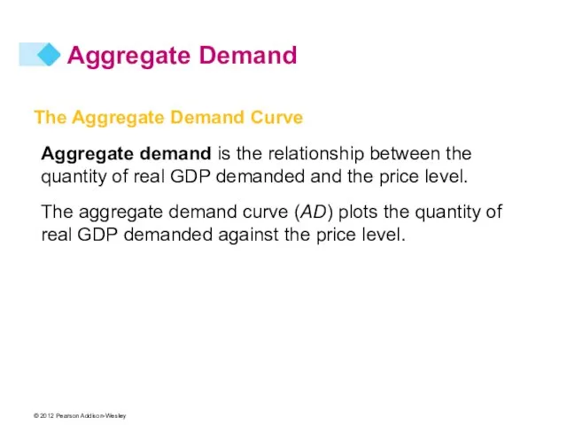
The Aggregate Demand Curve
Aggregate demand is the relationship between the quantity
Aggregate Demand
The Aggregate Demand Curve
Aggregate demand is the relationship between the quantity
Слайд 19Figure 10.4 shows an AD curve.
The AD curve slopes downward for two
Figure 10.4 shows an AD curve.
The AD curve slopes downward for two
Слайд 20Aggregate Demand
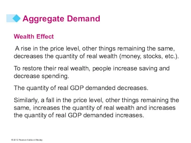
Wealth Effect
A rise in the price level, other things remaining
Aggregate Demand
Wealth Effect
A rise in the price level, other things remaining
Слайд 21Aggregate Demand
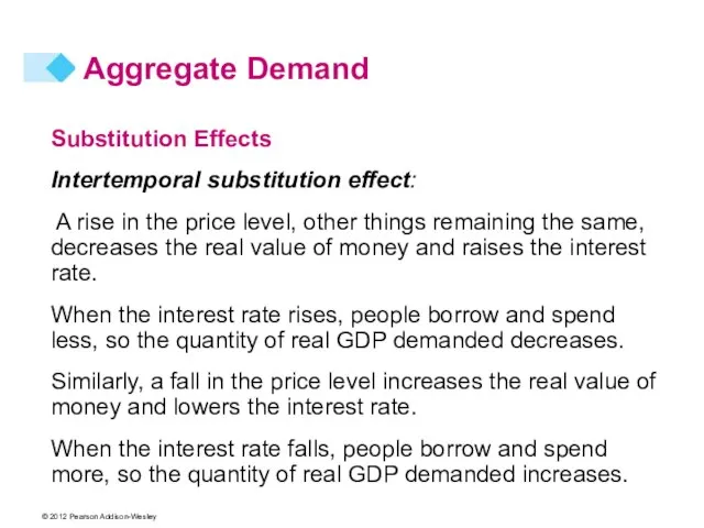
Substitution Effects
Intertemporal substitution effect:
A rise in the price level,
Aggregate Demand
Substitution Effects
Intertemporal substitution effect:
A rise in the price level,
Слайд 22Aggregate Demand
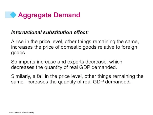
International substitution effect:
A rise in the price level, other things remaining
Aggregate Demand
International substitution effect:
A rise in the price level, other things remaining
Слайд 23Aggregate Demand
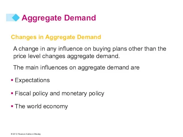
Changes in Aggregate Demand
A change in any influence on buying plans
Aggregate Demand
Changes in Aggregate Demand
A change in any influence on buying plans
Слайд 24Aggregate Demand
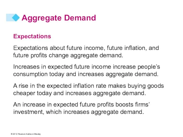
Expectations
Expectations about future income, future inflation, and future profits change aggregate
Aggregate Demand
Expectations
Expectations about future income, future inflation, and future profits change aggregate
Слайд 25Aggregate Demand
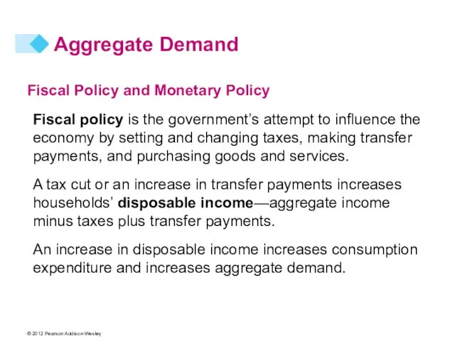
Fiscal Policy and Monetary Policy
Fiscal policy is the government’s attempt to
Aggregate Demand
Fiscal Policy and Monetary Policy
Fiscal policy is the government’s attempt to
Слайд 26Aggregate Demand
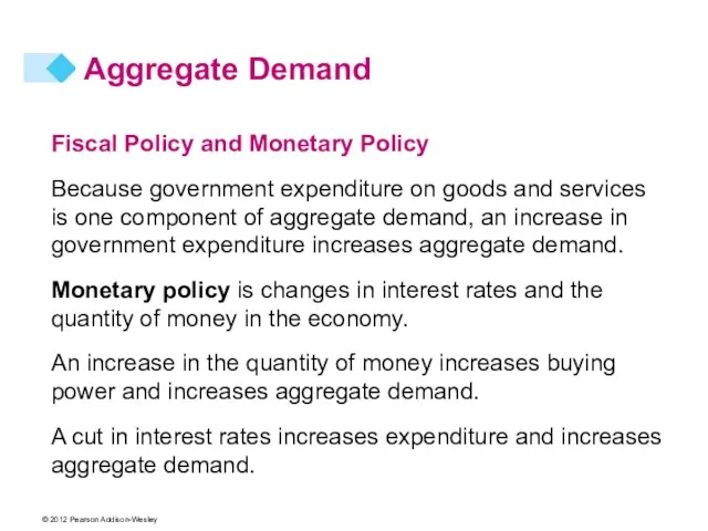
Fiscal Policy and Monetary Policy
Because government expenditure on goods and
Aggregate Demand
Fiscal Policy and Monetary Policy
Because government expenditure on goods and
Слайд 27Aggregate Demand
The World Economy
The world economy influences aggregate demand in two ways:
A
Aggregate Demand
The World Economy
The world economy influences aggregate demand in two ways:
A
Слайд 28Aggregate Demand
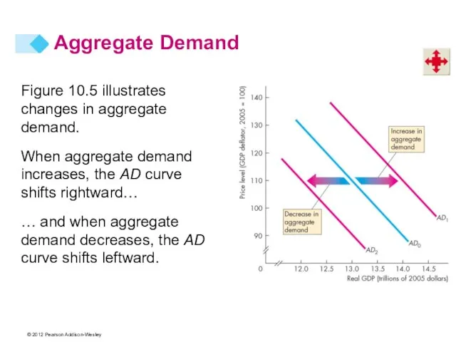
Figure 10.5 illustrates changes in aggregate demand.
When aggregate demand increases, the
Aggregate Demand
Figure 10.5 illustrates changes in aggregate demand.
When aggregate demand increases, the
Слайд 29Explaining Macroeconomic Trends and Fluctuations
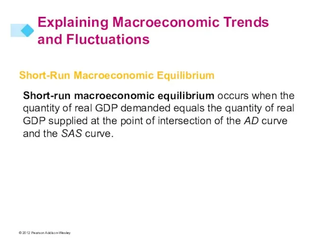
Short-Run Macroeconomic Equilibrium
Short-run macroeconomic equilibrium occurs when the
Explaining Macroeconomic Trends and Fluctuations
Short-Run Macroeconomic Equilibrium
Short-run macroeconomic equilibrium occurs when the
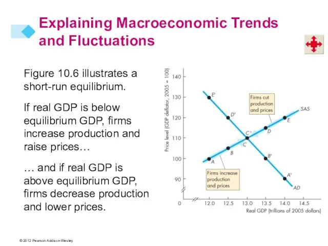
Слайд 30Figure 10.6 illustrates a short-run equilibrium.
If real GDP is below equilibrium GDP,
Figure 10.6 illustrates a short-run equilibrium.
If real GDP is below equilibrium GDP,
Слайд 31These changes bring a movement along the SAS curve towards equilibrium.
In short-run
These changes bring a movement along the SAS curve towards equilibrium.
In short-run
Слайд 32Long-Run Macroeconomic Equilibrium
Long-run macroeconomic equilibrium occurs when real GDP equals potential GDP—when
Long-Run Macroeconomic Equilibrium
Long-run macroeconomic equilibrium occurs when real GDP equals potential GDP—when
Слайд 33Figure 10.7 illustrates the adjustment to long-run equilibrium.
Initially, the economy is at
Figure 10.7 illustrates the adjustment to long-run equilibrium.
Initially, the economy is at
Слайд 34Initially, the economy is at an above-full employment equilibrium.
In the long run,
Initially, the economy is at an above-full employment equilibrium.
In the long run,
Слайд 35Economic Growth in the AS-AD Model
Figure 10.8 illustrates economic growth.
Because the quantity
Economic Growth in the AS-AD Model
Figure 10.8 illustrates economic growth.
Because the quantity
Слайд 36Figure 10.8 also illustrates inflation.
If the quantity of money grows faster than
Figure 10.8 also illustrates inflation.
If the quantity of money grows faster than
Слайд 37The Business Cycle in the AS-AD Model
The business cycle occurs because aggregate
The Business Cycle in the AS-AD Model
The business cycle occurs because aggregate
Слайд 38Figures 10.9(a) and (d) illustrate above full-employment equilibrium.
The amount by which potential
Figures 10.9(a) and (d) illustrate above full-employment equilibrium.
The amount by which potential
Слайд 39Figures 10.9(c) and (d)
illustrate below full-employment equilibrium.
The amount by which real
Figures 10.9(c) and (d)
illustrate below full-employment equilibrium.
The amount by which real
Слайд 40Fluctuations in Aggregate Demand
Figure 10.10 shows the effects of an increase in
Fluctuations in Aggregate Demand
Figure 10.10 shows the effects of an increase in
Слайд 41At the short-run equilibrium, there is an inflationary gap.
The money wage rate
At the short-run equilibrium, there is an inflationary gap.
The money wage rate
Слайд 42Fluctuations in Aggregate Supply
Figure 10.11 shows the effects of a rise in
Fluctuations in Aggregate Supply
Figure 10.11 shows the effects of a rise in

Слайд 43Macroeconomic Schools of Thought
Macroeconomists can be divided into three broad schools of
Macroeconomic Schools of Thought
Macroeconomists can be divided into three broad schools of
Слайд 44Macroeconomic Schools of Thought
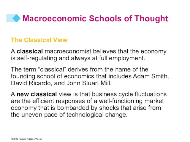
The Classical View
A classical macroeconomist believes that the economy
Macroeconomic Schools of Thought
The Classical View
A classical macroeconomist believes that the economy
Слайд 45Macroeconomic Schools of Thought
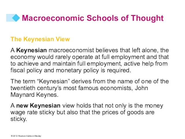
The Keynesian View
A Keynesian macroeconomist believes that left alone,
Macroeconomic Schools of Thought
The Keynesian View
A Keynesian macroeconomist believes that left alone,
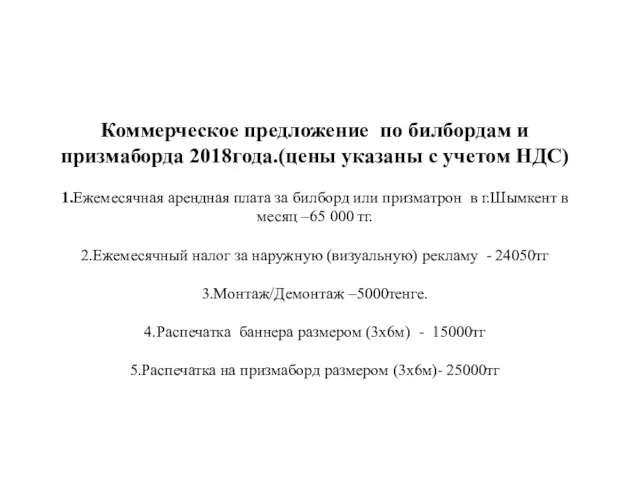 Коммерческое предложение по билбордам и призмаборда 2018 года
 Целеполагание в бизнесе
 Защита от несанкционированного доступа к информации
 15 минут про пиратство
 Агентство Brand Vision Republic - официальный партнёр ГО «Укрзалізниця»
 Мужской деловой костюм
 Презентация на тему Дети блокады
  Руководство для технического контент-менеджера
 ОРДЕНА И МЕДАЛИ ВЕЛИКОЙ ОТЕЧЕСТВЕННОЙ ВОЙНЫ
 Узкие места внутренней среды ООО Мясной гурман. Анализ ресурсов по Портеру
 Великие люди России. Александр Невский
 Модульное обучение на уроках русского языка
 Сибирский государственный университет геосистем и технологий. Научная жизнь кафедры экологии и природопользования
 Презентация на тему Праздник Новый Год
  По следам компьютерной мышки
 Российский флаг (3 класс)
 Почетный работник общего образования Российской Федерации Победитель конкурса лучших учителей Российской Федерации 2007г.
 Усгуги рекламы в Почте России
 День работника леса
 Всемирный Банк и МолодежьThe Young Professionals Program
 Путешествие в Древний Восток
 Морфологические нормы
 Время жить в Марий Эл
 Аттестация руководящих работников
 Антикафе
 Проповедь Христа
 Манипуляция
 Где логика. Пословицы и поговорки