- Linear Algebra. Lecture 2

Содержание
- 2. Learning Objectives: 1. Solving Homogeneous Systems. 2. Solving Nonhomogeneous Systems. 3. Applications. 4. Represent Linear Independence
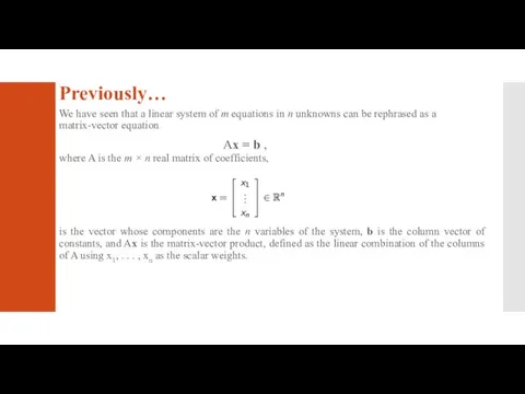
- 3. Previously… We have seen that a linear system of m equations in n unknowns can be
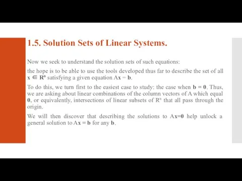
- 4. 1.5. Solution Sets of Linear Systems. Now we seek to understand the solution sets of such
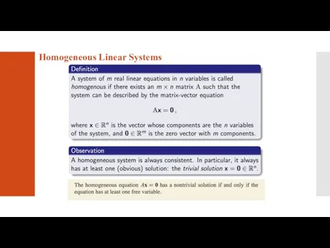
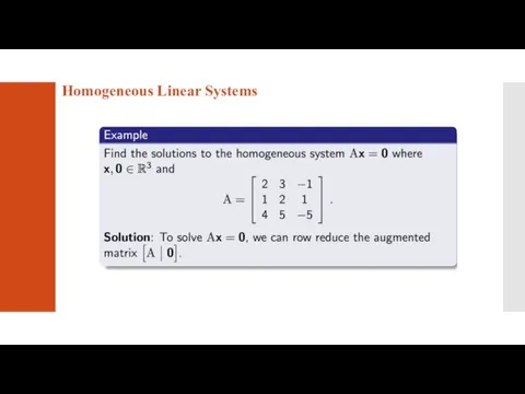
- 5. Homogeneous Linear Systems
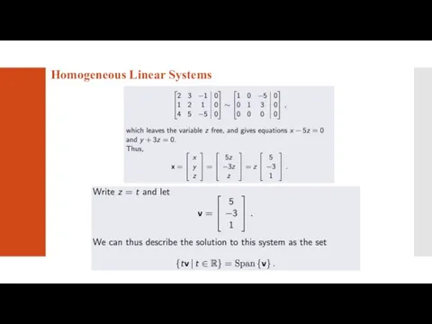
- 6. Homogeneous Linear Systems
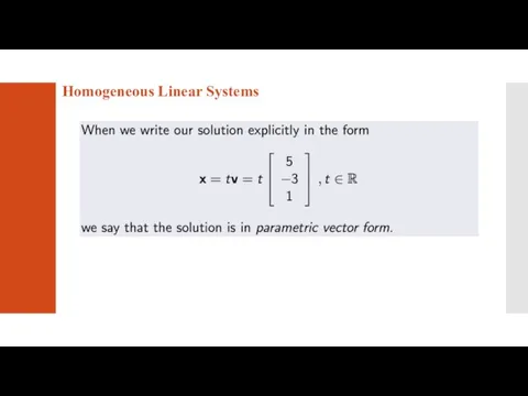
- 7. Homogeneous Linear Systems
- 8. Homogeneous Linear Systems
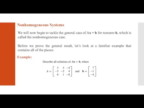
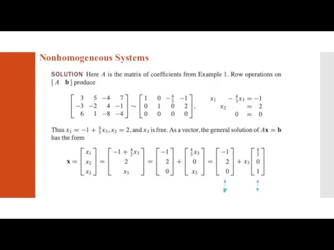
- 9. Nonhomogeneous Systems We will now begin to tackle the general case of Ax = b for
- 10. Nonhomogeneous Systems
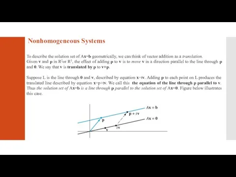
- 11. Nonhomogeneous Systems To describe the solution set of Ax=b geometrically, we can think of vector addition
- 12. Nonhomogeneous Systems
- 13. 1.6. Applications of Linear Algebra in SE Any applications in software engineering where a large amount
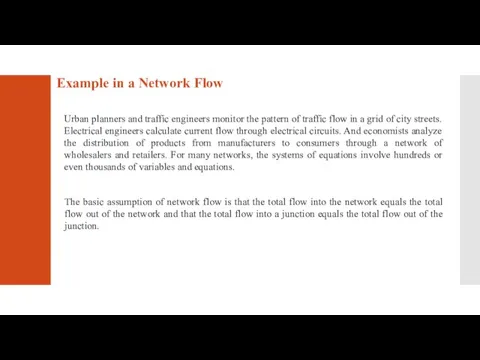
- 14. Example in a Network Flow Urban planners and traffic engineers monitor the pattern of traffic flow
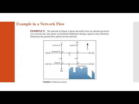
- 15. Example in a Network Flow
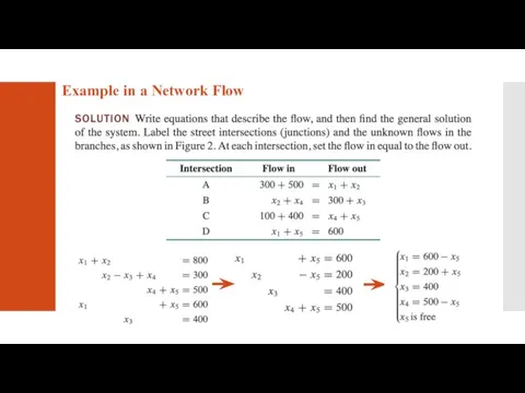
- 16. Example in a Network Flow
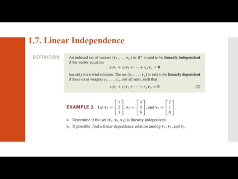
- 17. 1.7. Linear Independence
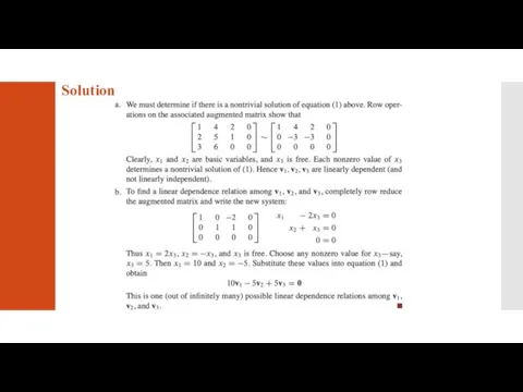
- 18. Solution
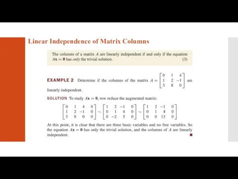
- 19. Linear Independence of Matrix Columns
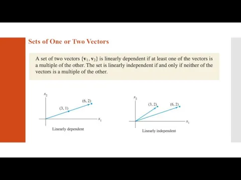
- 20. Sets of One or Two Vectors
- 21. Sets of Two or More Vectors
- 23. Скачать презентацию
Слайд 2Learning Objectives:
1. Solving Homogeneous Systems.
2. Solving Nonhomogeneous Systems.
3. Applications.
4. Represent
Learning Objectives: 1. Solving Homogeneous Systems. 2. Solving Nonhomogeneous Systems. 3. Applications. 4. Represent
Слайд 3Previously…
We have seen that a linear system of m equations in n
Previously…
We have seen that a linear system of m equations in n
Слайд 41.5. Solution Sets of Linear Systems.
Now we seek to understand the solution
1.5. Solution Sets of Linear Systems.
Now we seek to understand the solution
Слайд 5Homogeneous Linear Systems
Homogeneous Linear Systems
Слайд 6Homogeneous Linear Systems
Homogeneous Linear Systems
Слайд 7Homogeneous Linear Systems
Homogeneous Linear Systems
Слайд 8Homogeneous Linear Systems
Homogeneous Linear Systems
Слайд 9Nonhomogeneous Systems
We will now begin to tackle the general case of Ax
Nonhomogeneous Systems
We will now begin to tackle the general case of Ax
Слайд 10Nonhomogeneous Systems
Nonhomogeneous Systems
Слайд 11Nonhomogeneous Systems
To describe the solution set of Ax=b geometrically, we can think
Nonhomogeneous Systems
To describe the solution set of Ax=b geometrically, we can think
Слайд 12Nonhomogeneous Systems
Nonhomogeneous Systems
Слайд 131.6. Applications of Linear Algebra in SE
Any applications in software engineering where
1.6. Applications of Linear Algebra in SE
Any applications in software engineering where
Слайд 14Example in a Network Flow
Urban planners and traffic engineers monitor the pattern
Example in a Network Flow
Urban planners and traffic engineers monitor the pattern
Слайд 15Example in a Network Flow
Example in a Network Flow
Слайд 16Example in a Network Flow
Example in a Network Flow
Слайд 171.7. Linear Independence
1.7. Linear Independence
Слайд 18Solution
Solution
Слайд 19Linear Independence of Matrix Columns
Linear Independence of Matrix Columns
Слайд 20Sets of One or Two Vectors
Sets of One or Two Vectors
Слайд 21Sets of Two or More Vectors
Sets of Two or More Vectors

 Формирование действия моделирования через решение текстовых задач
 Võrratused Heldena Taperson
 Бесконечные периодические десятичные дроби
 Тригонометриялық теңдеулерді шешу тәсілдерін үйрену
 Радианная мера угла. Синус, косинус, тангенс числа
 Четырехугольники. Свойства четырехугольников. Решение задач
 Задачи на проценты
 Алгебра. Города
 Особенности применения средств измерений в качестве эталонов единицы величины
 Построение сечений
 Уровень и отвес
 Функция распределения дискретной случайной величины
 Презентация на тему НУМЕРАЦИИ РАЗНЫХ НАРОДОВ И ИХ ВОЗНИКНОВЕНИЕ
  Математика. Управление социальными системами. Математический анализ. Дифференцирование функции одной переменной
 Исследование функции с помощью производной
 Виды алгоритмов
 Система управління технологічного процесу приготування розчинів для піроксилінових порохів
 Многогранник с двумя основаниями
 Психолого – педагогические основы организации математического развития младших школьников
 Умножение дробей
 Многогранники
 Числа Фибоначчи
 Свойства биссектрисы угла. Решение задач
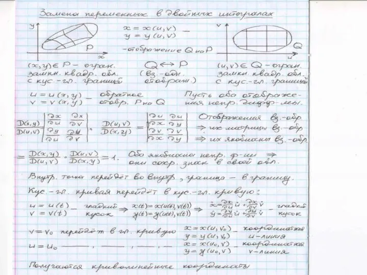 Замена переменных в двойных интегралах
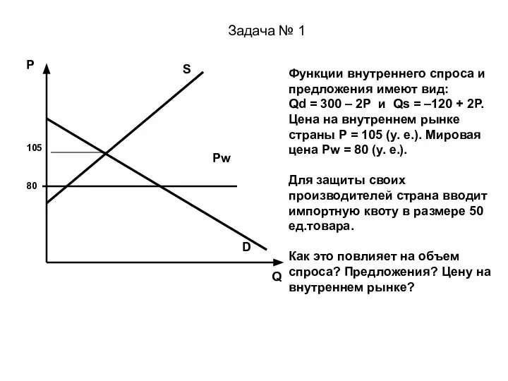 Функции внутреннего спроса и предложения. Разбор задач
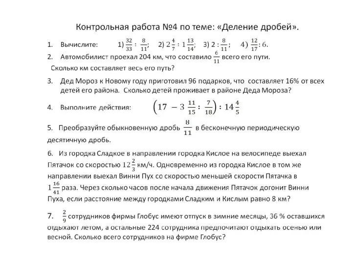 Деление дробей. Контрольная работа
 Порядок действий в выражениях со скобками
 Вариационный ряд. Группировка данных при качественной и количественной вариациях