- Credit and exam

Содержание
- 2. Mathematical models A mathematical model is a description of a system or problem using mathematical concepts,
- 3. Abstract algebra Algebraic structures Group, Abelian group Field Ring Vector space Vector space over a field
- 4. Linear algebra Vector space Vectors Components (coordinates) Basic operations Linear combination of vectors Linearly dependent or
- 5. Vector spaces Generators Basis Basis extension Steiner’s theorem
- 6. Matrices Type of matrix Matrix addition Matrix multiplication Scalar multiplication of matrix Inversion of square matrix
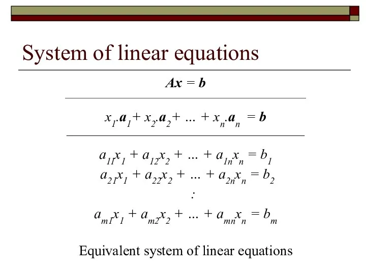
- 7. System of linear equations Ax = b _______________________________________________________________________________ x1.a1+ x2.a2+ … + xn.an = b ____________________________________________________
- 8. Solution of system of linear equations Gauss elimination Jordanian elimination Row echelon form Reduced row echelon
- 9. Jordanian elimination Elementary row (column) operation Exchange the rows Multiplying row by a scalar Add one
- 10. Solubility of system of linear equations The system has no solution (in this case, we say
- 11. Mathematical programming Optimization model min {f(x) ⏐ qi(x) ≤ 0 , i = 1, ..., m
- 12. General optimality problems Feasibility problem The satisfiability problem, also called the feasibility problem, is just the
- 13. Classification of optimization models More then one constraint Number of criteria Single optimization Multiple optimization Type
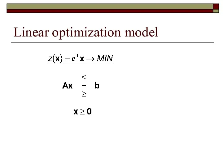
- 14. Linear optimization model
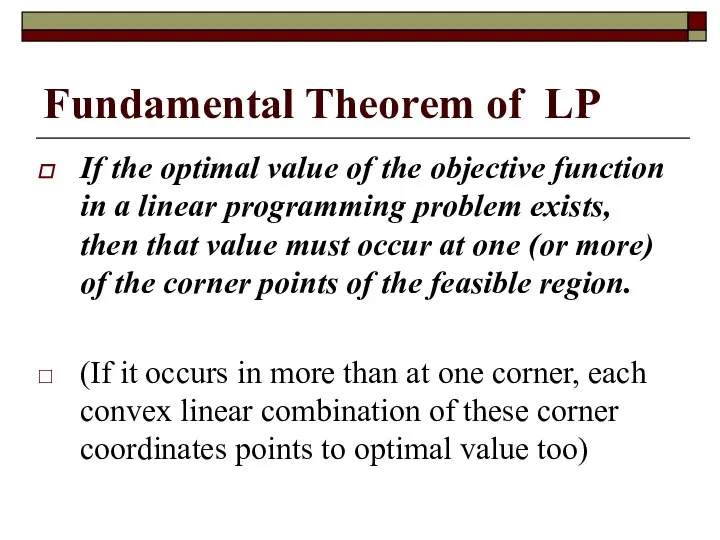
- 15. Fundamental Theorem of LP If the optimal value of the objective function in a linear programming
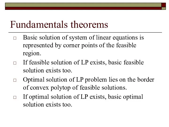
- 16. Fundamentals theorems Basic solution of system of linear equations is represented by corner points of the
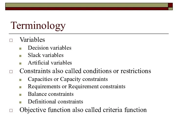
- 17. Terminology Variables Decision variables Slack variables Artificial variables Constraints also called conditions or restrictions Capacities or
- 18. Terminology Feasible solution – feasibility region, search space, choice set Basic solution Infeasible solution Optimal solution
- 19. Existence of solution Nonexistence of solution If the feasible region is empty (that is, there are
- 20. Matrices as basic vectors Column space of a matrix is the set of all possible linear
- 21. Graphical representation I Convex polytop Bounded Unbounded
- 22. Graphical representation II Column space of matrix of coefficients
- 23. Simplex Method Simplex method Starts with a feasible solution Tests whether or not it is optimum.
- 24. The Simplex Algorithm
- 25. The Simplex Algorithm Converting LP into standard and canonical form Definition of slack variables Definition of
- 26. Solubility of linear model One optimal solution Infinite number of optimal solution Alternate solutions - If
- 27. Simple transportation problem Suppliers, source – supply of i-th supplier ai Demands, destinations – demand of
- 28. Transportation table
- 29. Balanced transportation model Σj xij = ai , i=1,…,m Σi xij = bj , j=1,…,n xij
- 30. Balanced transportation system Total supply = total demand Σj ai = Σj bj dummy supplier dummy
- 31. Solving of the TP Initial solution must be feasible Northwest-Corner method (NWCM) Least-Cost method (LCM) Vogel's
- 32. Transportation method Step 0 – Balanced transportation system Step 1 – Initial basic solution Step 2
- 33. Degeneracy The basic solution is degenerate if some of basic variables is equal to zero. Degeneracy
- 34. Result analysis Optimal solution Alternative solution Suboptimal solution Perspective routes Routes substitution Possible shipped amount
- 35. Vehicle routing problem Given a list of cities and their pairwise distances The task is to
- 36. Travelling salesman problem Given a list of cities and their pairwise distances The task is to
- 37. Solving of TSP Try all permutations of points N! possibilities Principle: adding of branches to pass
- 38. Vehicle routing problem Majer‘s method Central point Selecting the most distant point from the central point
- 39. Game Model of conflict or competition Cooperative, non-cooperative games Antagonistic – non-antagonistic game Time – simultaneous
- 40. Solution of game Each player tries to maximize his welfare at the expense of the others.
- 41. Model of game Tree (extensive) form of model Game tree (decision tree - moves) Normal form
- 42. Matrix game Two-person game Finite number of strategies for each player Zero-sum game Sum of payoffs
- 43. Pure and mixed strategy Pure strategy One best strategy How to find it – saddle point
- 44. Matrix game solution Theorem The optimal pure strategies exist in the matrix game, if and only
- 45. Decision model Model elements Decision alternatives States of nature Decision matrix (table) – payoffs associated with
- 46. Solution of decision problems Selection of the dominating alternative Selection of the best alternative Selection of
- 47. Selection of the dominating alternative Outcome dominance: aI dominates aK Event dominance: aI dominates aK Probabilistic
- 48. Selection of the best alternative Decision-making under certainty Decision-making under uncertainty Maximax rule Wald criterion -
- 49. Multiple Objective Decision Making Infinite Number of Alternatives At least two criteria Example – Linear multi
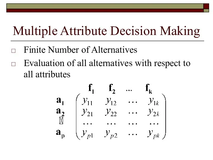
- 50. Multiple Attribute Decision Making Finite Number of Alternatives Evaluation of all alternatives with respect to all
- 51. Basic terms Ideal alternative Nadir alternative Dominating and dominated alternative The best alternative – preferred alternative
- 52. The aim of MADM Selection of the best alternatives (one or more) Dichotomizing into the efficient
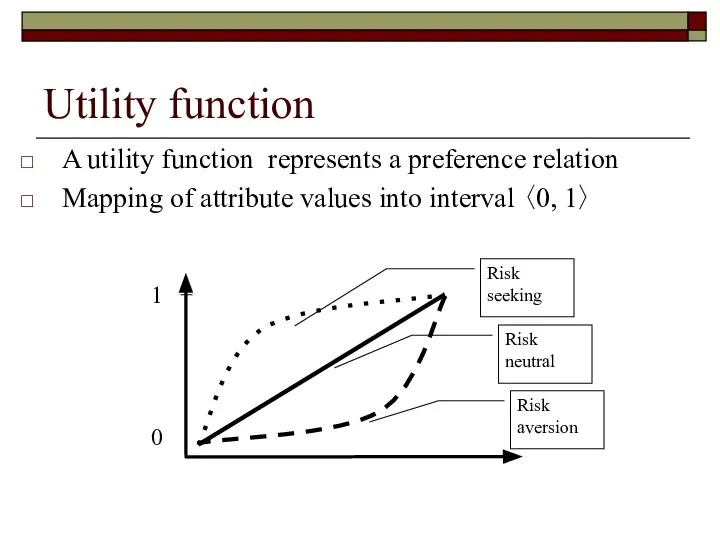
- 53. Utility, utility function Utility is a measure of satisfaction All attribute values can be expresed by
- 54. Utility function A utility function represents a preference relation Mapping of attribute values into interval 〈0,
- 55. Informations Inter and intra attribute comparisons Criteria preferences Alternatives preferences Not necessary in numerical form No
- 56. Methods for assesing information Sequence Method Criteria/alternatives are arranged according their importance to a sequence from
- 57. MADM methods Scoring or sequence methods Standard level methods Simple additive weighting method Attributes must be
- 59. Скачать презентацию
Слайд 3Abstract algebra
Algebraic structures
Group, Abelian group
Field
Ring
Vector space
Vector space over a field F
Abstract algebra
Algebraic structures
Group, Abelian group
Field
Ring
Vector space
Vector space over a field F
Слайд 4Linear algebra
Vector space
Vectors
Components (coordinates)
Basic operations
Linear combination of vectors
Linearly dependent or independent
Linear algebra
Vector space
Vectors
Components (coordinates)
Basic operations
Linear combination of vectors
Linearly dependent or independent
Слайд 5Vector spaces
Generators
Basis
Basis extension
Steiner’s theorem
Vector spaces
Generators
Basis
Basis extension
Steiner’s theorem
Слайд 6Matrices
Type of matrix
Matrix addition
Matrix multiplication
Scalar multiplication of matrix
Inversion of square matrix
Rank of
Matrices
Type of matrix
Matrix addition
Matrix multiplication
Scalar multiplication of matrix
Inversion of square matrix
Rank of
Слайд 7System of linear equations
Ax = b
_______________________________________________________________________________
x1.a1+ x2.a2+ … + xn.an =
System of linear equations
Ax = b
_______________________________________________________________________________
x1.a1+ x2.a2+ … + xn.an =
Слайд 8Solution of system of linear equations
Gauss elimination
Jordanian elimination
Row echelon form
Reduced row echelon
Solution of system of linear equations
Gauss elimination
Jordanian elimination
Row echelon form
Reduced row echelon
Слайд 9Jordanian elimination
Elementary row (column) operation
Exchange the rows
Multiplying row by a scalar
Add one
Jordanian elimination
Elementary row (column) operation
Exchange the rows
Multiplying row by a scalar
Add one
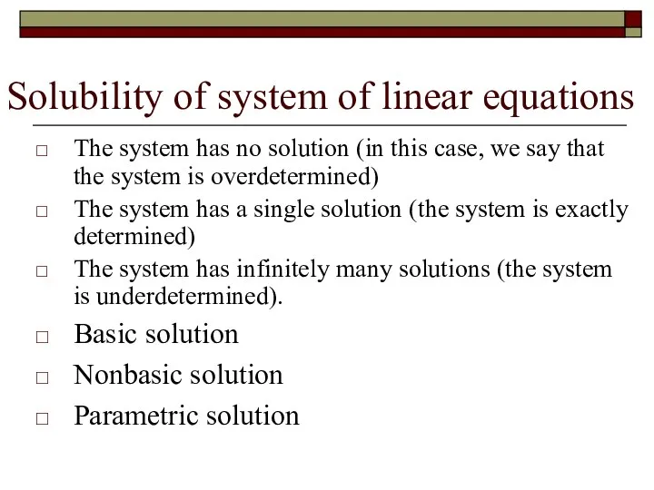
Слайд 10Solubility of system of linear equations
The system has no solution (in this
Solubility of system of linear equations
The system has no solution (in this
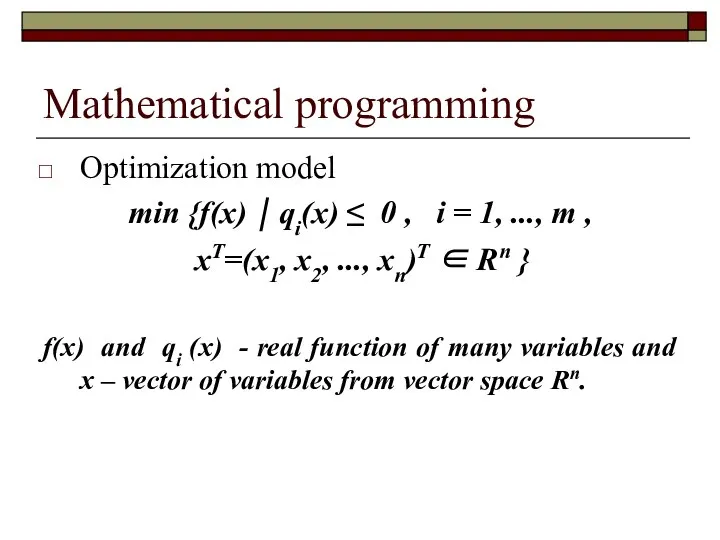
Слайд 11Mathematical programming
Optimization model
min {f(x) ⏐ qi(x) ≤ 0 , i = 1,
Mathematical programming
Optimization model
min {f(x) ⏐ qi(x) ≤ 0 , i = 1,
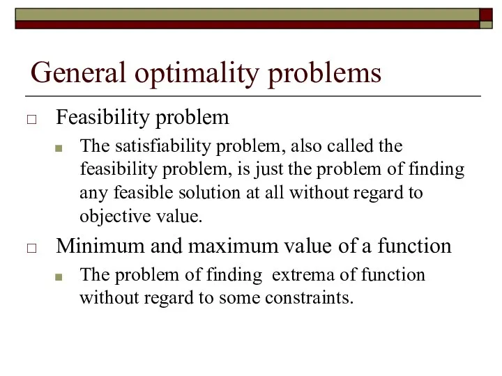
Слайд 12General optimality problems
Feasibility problem
The satisfiability problem, also called the feasibility problem, is
General optimality problems
Feasibility problem
The satisfiability problem, also called the feasibility problem, is
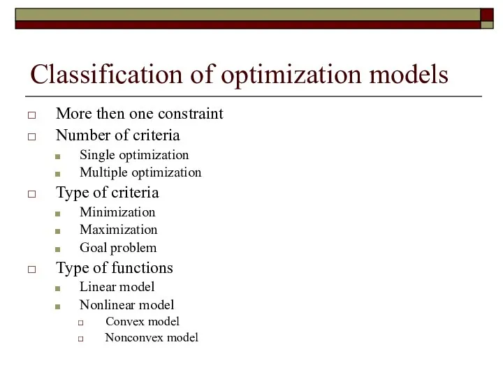
Слайд 13Classification of optimization models
More then one constraint
Number of criteria
Single optimization
Multiple optimization
Type
Classification of optimization models
More then one constraint
Number of criteria
Single optimization
Multiple optimization
Type
Слайд 14Linear optimization model
Linear optimization model
Слайд 15Fundamental Theorem of LP
If the optimal value of the objective function in
Fundamental Theorem of LP
If the optimal value of the objective function in
Слайд 16Fundamentals theorems
Basic solution of system of linear equations is represented by corner
Fundamentals theorems
Basic solution of system of linear equations is represented by corner
Слайд 17Terminology
Variables
Decision variables
Slack variables
Artificial variables
Constraints also called conditions or restrictions
Capacities or Capacity
Terminology
Variables
Decision variables
Slack variables
Artificial variables
Constraints also called conditions or restrictions
Capacities or Capacity
Слайд 18Terminology
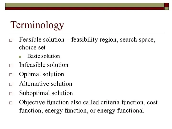
Feasible solution – feasibility region, search space, choice set
Basic solution
Infeasible solution
Optimal solution
Alternative
Terminology
Feasible solution – feasibility region, search space, choice set
Basic solution
Infeasible solution
Optimal solution
Alternative
Слайд 19Existence of solution
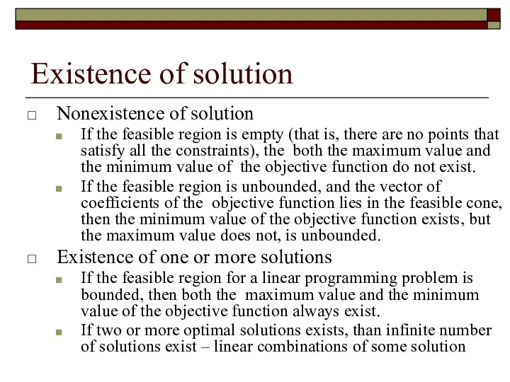
Nonexistence of solution
If the feasible region is empty (that is,
Existence of solution
Nonexistence of solution
If the feasible region is empty (that is,
Слайд 20Matrices as basic vectors
Column space of a matrix is the set of
Matrices as basic vectors
Column space of a matrix is the set of
Слайд 21Graphical representation I
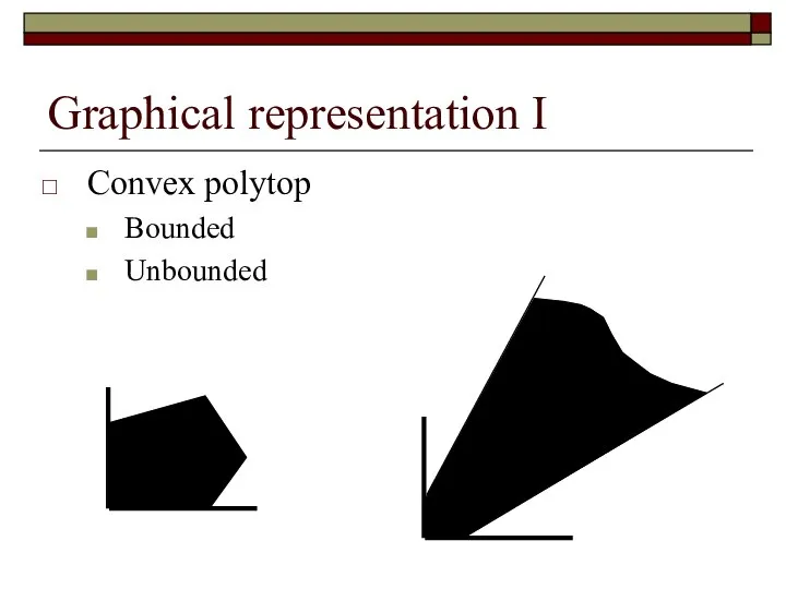
Convex polytop
Bounded
Unbounded
Graphical representation I
Convex polytop
Bounded
Unbounded
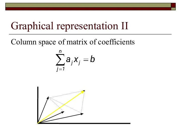
Слайд 22Graphical representation II
Column space of matrix of coefficients
Graphical representation II
Column space of matrix of coefficients
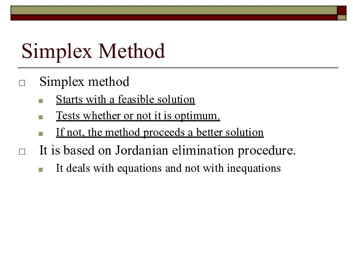
Слайд 23Simplex Method
Simplex method
Starts with a feasible solution
Tests whether or not
Simplex Method
Simplex method
Starts with a feasible solution
Tests whether or not
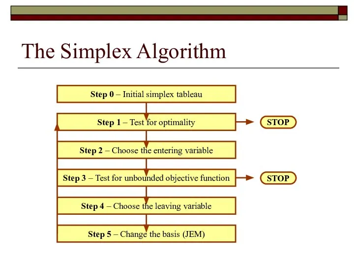
Слайд 24The Simplex Algorithm
The Simplex Algorithm
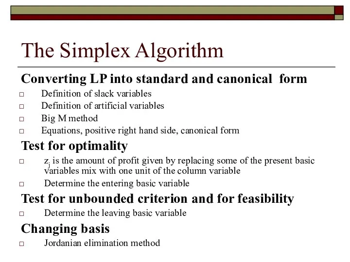
Слайд 25The Simplex Algorithm
Converting LP into standard and canonical form
Definition of slack variables
Definition
The Simplex Algorithm
Converting LP into standard and canonical form
Definition of slack variables
Definition
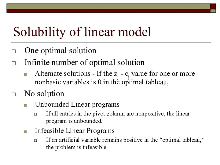
Слайд 26Solubility of linear model
One optimal solution
Infinite number of optimal solution
Alternate solutions -
Solubility of linear model
One optimal solution
Infinite number of optimal solution
Alternate solutions -
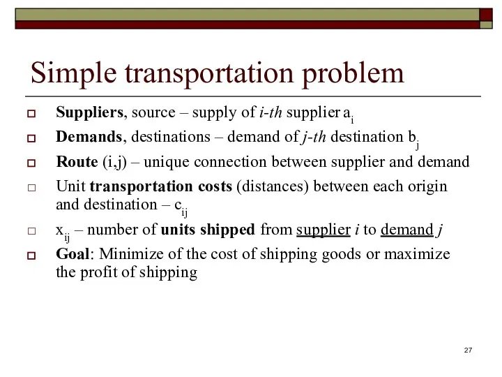
Слайд 27Simple transportation problem
Suppliers, source – supply of i-th supplier ai
Demands, destinations –
Simple transportation problem
Suppliers, source – supply of i-th supplier ai
Demands, destinations –
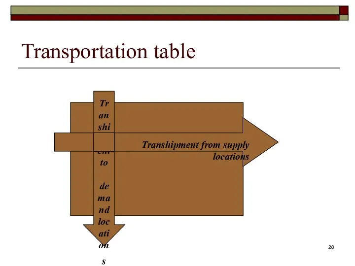
Слайд 28Transportation table
Transportation table
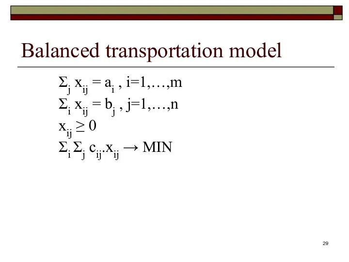
Слайд 29Balanced transportation model
Σj xij = ai , i=1,…,m
Σi xij = bj ,
Balanced transportation model
Σj xij = ai , i=1,…,m
Σi xij = bj ,
Слайд 30Balanced transportation system
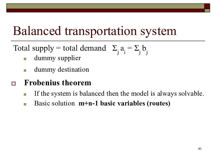
Total supply = total demand Σj ai = Σj bj
Balanced transportation system
Total supply = total demand Σj ai = Σj bj
Слайд 31Solving of the TP
Initial solution must be feasible
Northwest-Corner method (NWCM)
Least-Cost method (LCM)
Vogel's
Solving of the TP
Initial solution must be feasible
Northwest-Corner method (NWCM)
Least-Cost method (LCM)
Vogel's
Слайд 32Transportation method
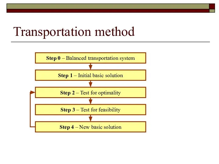
Step 0 – Balanced transportation system
Step 1 – Initial basic
Transportation method
Step 0 – Balanced transportation system
Step 1 – Initial basic
Слайд 33Degeneracy
The basic solution is degenerate if some of basic variables is equal
Degeneracy
The basic solution is degenerate if some of basic variables is equal
Слайд 34Result analysis
Optimal solution
Alternative solution
Suboptimal solution
Perspective routes
Routes substitution
Possible shipped amount
Result analysis
Optimal solution
Alternative solution
Suboptimal solution
Perspective routes
Routes substitution
Possible shipped amount
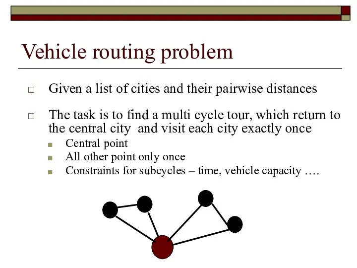
Слайд 35Vehicle routing problem
Given a list of cities and their pairwise distances
The task
Vehicle routing problem
Given a list of cities and their pairwise distances
The task
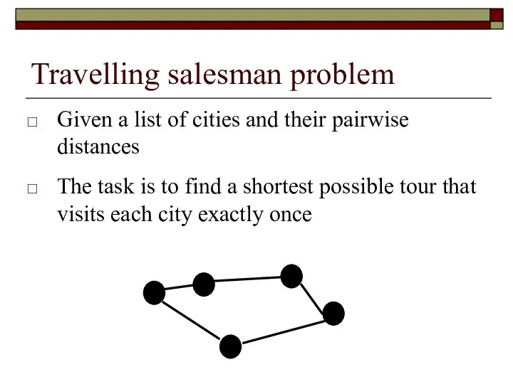
Слайд 36Travelling salesman problem
Given a list of cities and their pairwise distances
The
Travelling salesman problem
Given a list of cities and their pairwise distances
The
Слайд 37Solving of TSP
Try all permutations of points
N! possibilities
Principle: adding of branches to
Solving of TSP
Try all permutations of points
N! possibilities
Principle: adding of branches to
Слайд 38Vehicle routing problem
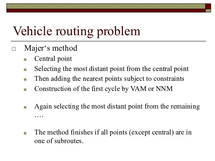
Majer‘s method
Central point
Selecting the most distant point from the central
Vehicle routing problem
Majer‘s method
Central point
Selecting the most distant point from the central
Слайд 39Game
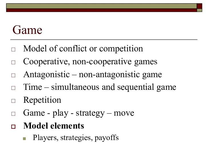
Model of conflict or competition
Cooperative, non-cooperative games
Antagonistic – non-antagonistic game
Time – simultaneous
Game
Model of conflict or competition
Cooperative, non-cooperative games
Antagonistic – non-antagonistic game
Time – simultaneous
Слайд 40Solution of game
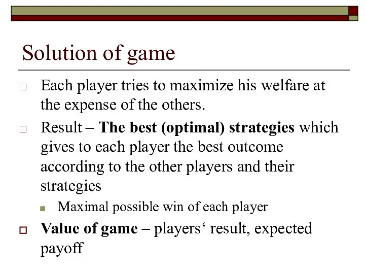
Each player tries to maximize his welfare at the expense
Solution of game
Each player tries to maximize his welfare at the expense
Слайд 41Model of game
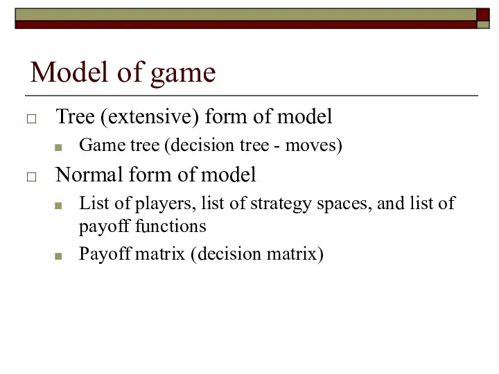
Tree (extensive) form of model
Game tree (decision tree - moves)
Normal
Model of game
Tree (extensive) form of model
Game tree (decision tree - moves)
Normal
Слайд 42Matrix game
Two-person game
Finite number of strategies for each player
Zero-sum game
Sum of payoffs
Matrix game
Two-person game
Finite number of strategies for each player
Zero-sum game
Sum of payoffs
Слайд 43Pure and mixed strategy
Pure strategy
One best strategy
How to find it – saddle
Pure and mixed strategy
Pure strategy
One best strategy
How to find it – saddle
Слайд 44Matrix game solution
Theorem
The optimal pure strategies exist in the matrix game, if
Matrix game solution
Theorem
The optimal pure strategies exist in the matrix game, if
Слайд 45Decision model
Model elements
Decision alternatives
States of nature
Decision matrix (table) – payoffs associated with
Decision model
Model elements
Decision alternatives
States of nature
Decision matrix (table) – payoffs associated with
Слайд 46Solution of decision problems
Selection of the dominating alternative
Selection of the best
Solution of decision problems
Selection of the dominating alternative
Selection of the best
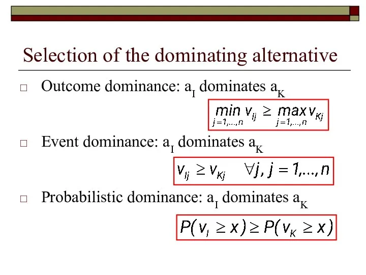
Слайд 47Selection of the dominating alternative
Outcome dominance: aI dominates aK
Event dominance: aI dominates
Selection of the dominating alternative
Outcome dominance: aI dominates aK
Event dominance: aI dominates
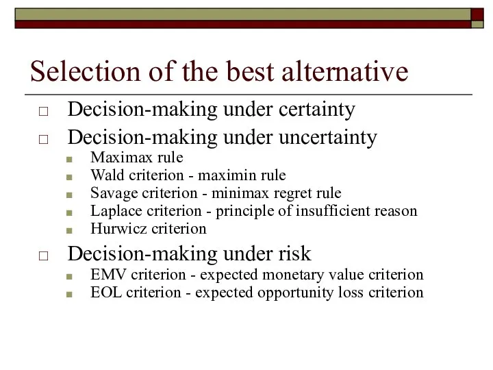
Слайд 48Selection of the best alternative
Decision-making under certainty
Decision-making under uncertainty
Maximax rule
Wald criterion -
Selection of the best alternative
Decision-making under certainty
Decision-making under uncertainty
Maximax rule
Wald criterion -
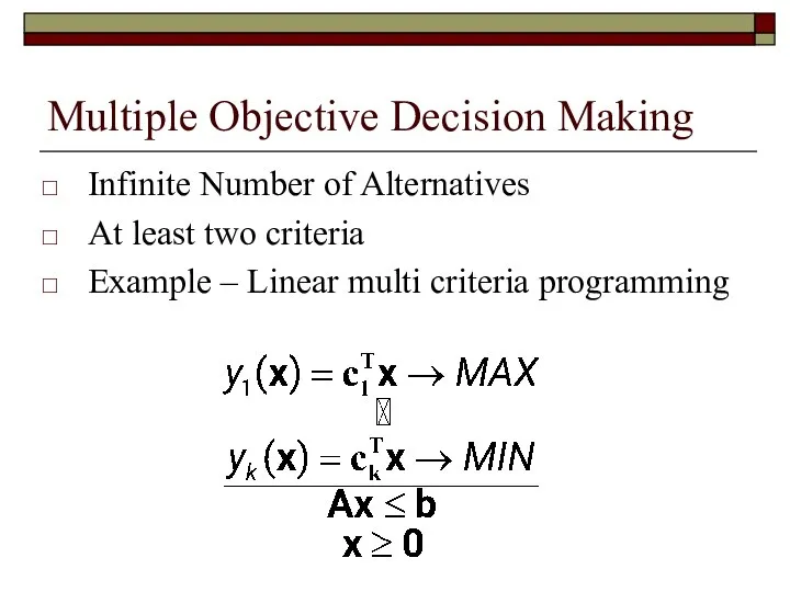
Слайд 49Multiple Objective Decision Making
Infinite Number of Alternatives
At least two criteria
Example – Linear
Multiple Objective Decision Making
Infinite Number of Alternatives
At least two criteria
Example – Linear
Слайд 50Multiple Attribute Decision Making
Finite Number of Alternatives
Evaluation of all alternatives with respect
Multiple Attribute Decision Making
Finite Number of Alternatives
Evaluation of all alternatives with respect
Слайд 51Basic terms
Ideal alternative
Nadir alternative
Dominating and dominated alternative
The best alternative – preferred alternative
Pareto
Basic terms
Ideal alternative
Nadir alternative
Dominating and dominated alternative
The best alternative – preferred alternative
Pareto
Слайд 52The aim of MADM
Selection of the best alternatives (one or more)
Dichotomizing into
The aim of MADM
Selection of the best alternatives (one or more)
Dichotomizing into
Слайд 53Utility, utility function
Utility is a measure of satisfaction
All attribute values can
Utility, utility function
Utility is a measure of satisfaction
All attribute values can
Слайд 54Utility function
A utility function represents a preference relation
Mapping of attribute values
Utility function
A utility function represents a preference relation
Mapping of attribute values
Слайд 55Informations
Inter and intra attribute comparisons
Criteria preferences
Alternatives preferences
Not necessary in numerical form
No preference
Informations
Inter and intra attribute comparisons
Criteria preferences
Alternatives preferences
Not necessary in numerical form
No preference
Слайд 56Methods for assesing information
Sequence Method
Criteria/alternatives are arranged according their importance to
Methods for assesing information
Sequence Method
Criteria/alternatives are arranged according their importance to
Слайд 57MADM methods
Scoring or sequence methods
Standard level methods
Simple additive weighting method
Attributes must be
MADM methods
Scoring or sequence methods
Standard level methods
Simple additive weighting method
Attributes must be
 Соответствия величин вычисления. 11 класс, 9 задание
 Линейные пространства и подпространства
 Сложение и вычитание смешанных чисел. Подготовка к контрольной работе
 Решение задач на увеличение и уменьшение числа на несколько единиц
 Двойственные задачи линейного программирования. Лекция 3
 Математическая разминка
 Производная. Физический смысл производной. Приращение аргумента и приращение функции. Задания
 Комплексные числа. Все формы
 2_Calculations
 Логарифмические неравенства
 Из истории геометрии
 Основы метрологии. Лекция 1
 Взаимное расположение графиков линейных функций
 Деление десятичной дроби на натуральное число
 Геометрические фигуры
 Линейное уравнение с одной переменной, содержащее знак модуля
 Учебный проект Чудесные дроби. 6 класс
 Геометрическая прогрессия
 Пересечение двух поверхностей. Построение пересечения двух кривых поверхностей методом плоских посредников
 Решение примеров в пределах 10
 Наибольшее и наименьшее значение функций
 Найдите объем тела вращения вокруг оси 0х , ограниченной прямыми
 РўР’РёРњРЎ_Лекция 2_Теоремы Рѕ вероятностях СЃРожных событий (4)
 Фундаментальная система решений (ФСР)
 Презентация на тему Площадь четырёхугольника
  Стереометрия. Метод координат в задачах ЕГЭ
 Теорема синусов и косинусов
 Взаимное расположение сферы и плоскости