- Probability Distributions

Содержание
- 2. Random Variable A random variable x takes on a defined set of values with different probabilities.
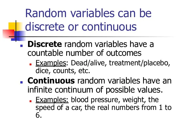
- 3. Random variables can be discrete or continuous Discrete random variables have a countable number of outcomes
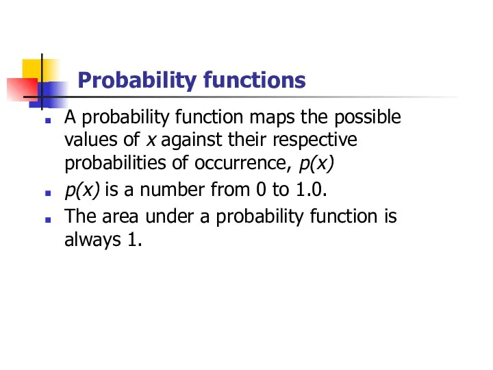
- 4. Probability functions A probability function maps the possible values of x against their respective probabilities of
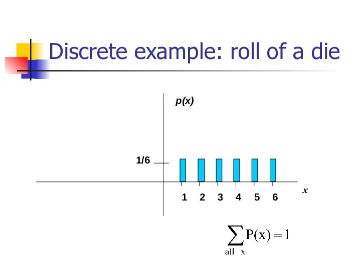
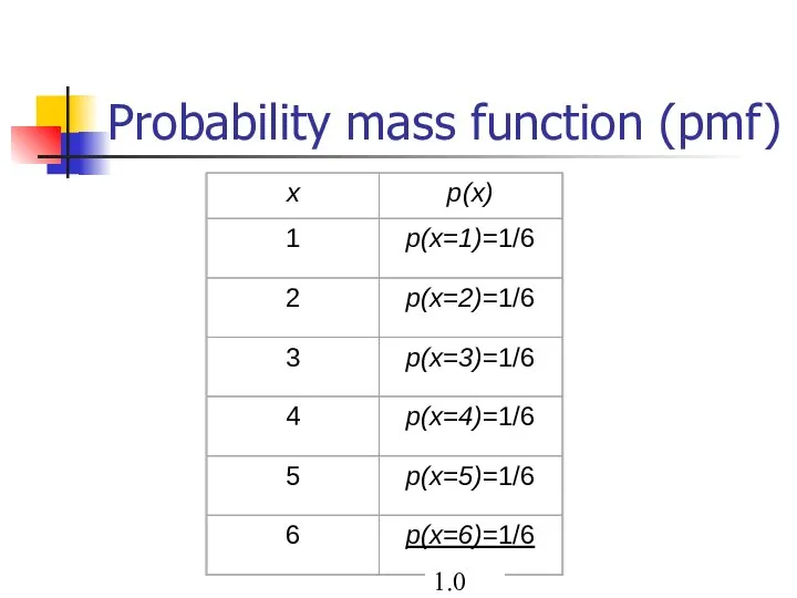
- 5. Discrete example: roll of a die
- 6. Probability mass function (pmf)
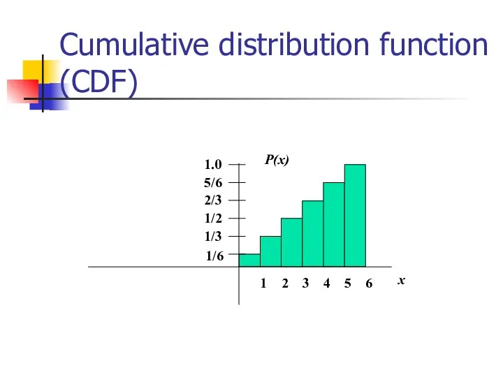
- 7. Cumulative distribution function (CDF)
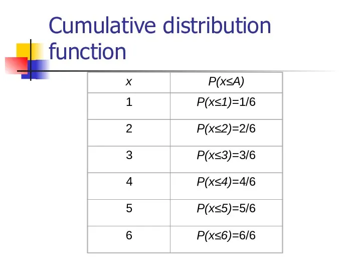
- 8. Cumulative distribution function
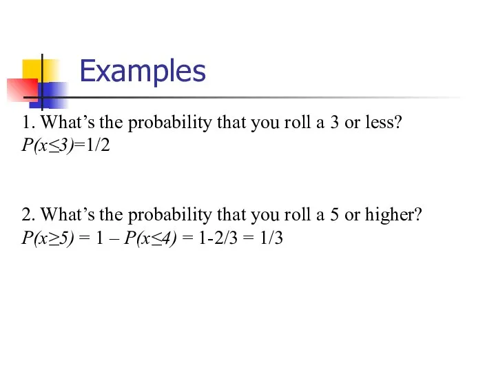
- 9. Examples 1. What’s the probability that you roll a 3 or less? P(x≤3)=1/2 2. What’s the
- 10. Practice Problem Which of the following are probability functions? a. f(x)=.25 for x=9,10,11,12 b. f(x)= (3-x)/2
- 11. Answer (a) a. f(x)=.25 for x=9,10,11,12 1.0
- 12. Answer (b) b. f(x)= (3-x)/2 for x=1,2,3,4
- 13. Answer (c) c. f(x)= (x2+x+1)/25 for x=0,1,2,3
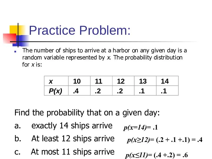
- 14. Practice Problem: The number of ships to arrive at a harbor on any given day is
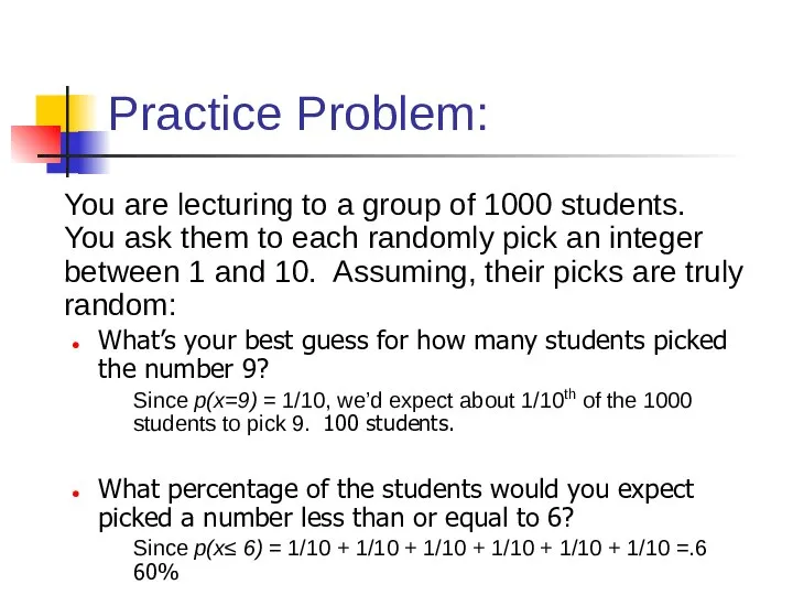
- 15. Practice Problem: You are lecturing to a group of 1000 students. You ask them to each
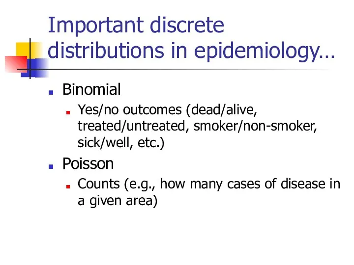
- 16. Important discrete distributions in epidemiology… Binomial Yes/no outcomes (dead/alive, treated/untreated, smoker/non-smoker, sick/well, etc.) Poisson Counts (e.g.,
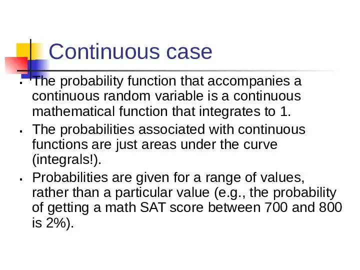
- 17. Continuous case The probability function that accompanies a continuous random variable is a continuous mathematical function
- 18. Continuous case For example, recall the negative exponential function (in probability, this is called an “exponential
- 19. Continuous case: “probability density function” (pdf) The probability that x is any exact particular value (such
- 20. For example, the probability of x falling within 1 to 2:
- 21. Cumulative distribution function As in the discrete case, we can specify the “cumulative distribution function” (CDF):
- 22. Example
- 23. Example 2: Uniform distribution The uniform distribution: all values are equally likely The uniform distribution: f(x)=
- 24. Example: Uniform distribution What’s the probability that x is between ¼ and ½? P(½ ≥x≥ ¼
- 25. Practice Problem 4. Suppose that survival drops off rapidly in the year following diagnosis of a
- 26. Answer The probability of dying within 1 year can be calculated using the cumulative distribution function:
- 27. Expected Value and Variance All probability distributions are characterized by an expected value and a variance
- 28. For example, bell-curve (normal) distribution:
- 29. Expected value, or mean If we understand the underlying probability function of a certain phenomenon, then
- 30. Example: expected value Recall the following probability distribution of ship arrivals:
- 31. Expected value, formally Discrete case: Continuous case:
- 32. Empirical Mean is a special case of Expected Value… Sample mean, for a sample of n
- 33. Expected value, formally Discrete case: Continuous case:
- 34. Extension to continuous case: uniform distribution x p(x) 1 1
- 35. Symbol Interlude E(X) = µ these symbols are used interchangeably
- 36. Expected Value Expected value is an extremely useful concept for good decision-making!
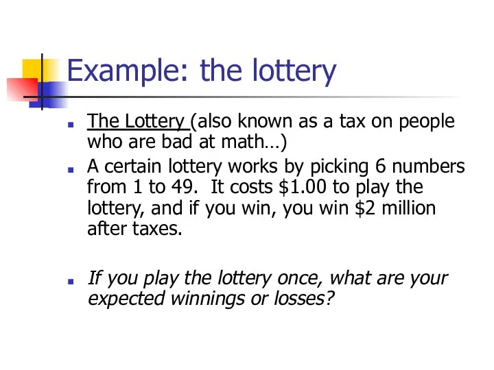
- 37. Example: the lottery The Lottery (also known as a tax on people who are bad at
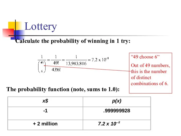
- 38. Lottery Calculate the probability of winning in 1 try: The probability function (note, sums to 1.0):
- 39. Expected Value The probability function Expected Value E(X) = P(win)*$2,000,000 + P(lose)*-$1.00 = 2.0 x 10⁶
- 40. Expected Value If you play the lottery every week for 10 years, what are your expected
- 41. Gambling (or how casinos can afford to give so many free drinks…) A roulette wheel has
- 42. **A few notes about Expected Value as a mathematical operator: If c= a constant number (i.e.,
- 43. E(c) = c E(c) = c Example: If you cash in soda cans in CA, you
- 44. E(cX)=cE(X) E(cX)=cE(X) Example: If the casino charges $10 per game instead of $1, then the casino
- 45. E(c + X)=c + E(X) E(c + X)=c + E(X) Example, if the casino throws in
- 46. E(X+Y)= E(X) + E(Y) E(X+Y)= E(X) + E(Y) Example: If you play the lottery twice, you
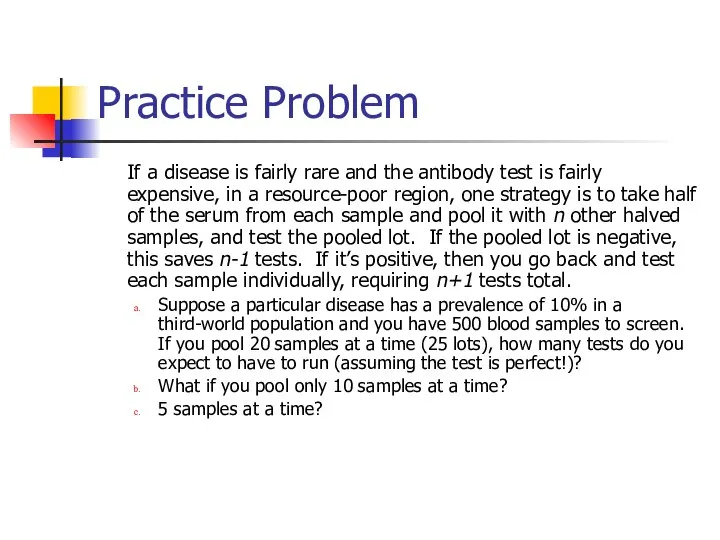
- 47. Practice Problem If a disease is fairly rare and the antibody test is fairly expensive, in
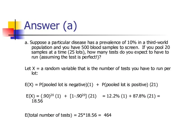
- 48. Answer (a) a. Suppose a particular disease has a prevalence of 10% in a third-world population
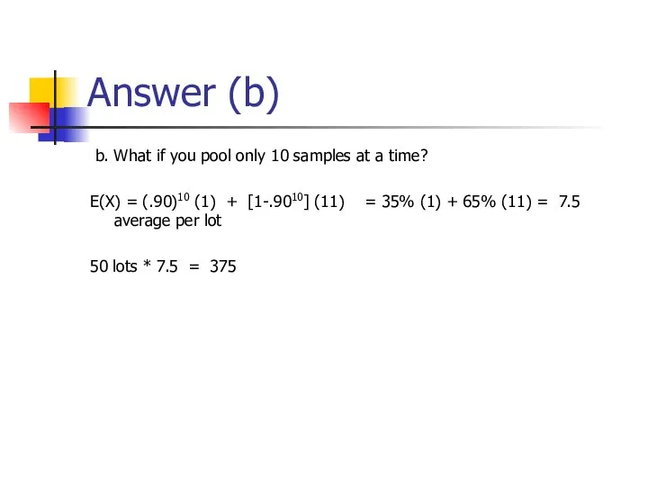
- 49. Answer (b) b. What if you pool only 10 samples at a time? E(X) = (.90)10
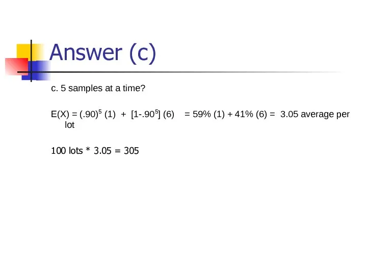
- 50. Answer (c) c. 5 samples at a time? E(X) = (.90)5 (1) + [1-.905] (6) =
- 51. Practice Problem If X is a random integer between 1 and 10, what’s the expected value
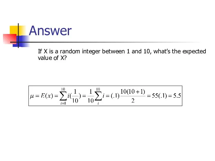
- 52. Answer If X is a random integer between 1 and 10, what’s the expected value of
- 53. Expected value isn’t everything though… Take the show “Deal or No Deal” Everyone know the rules?
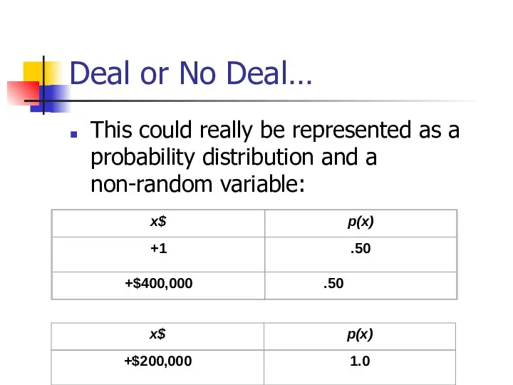
- 54. Deal or No Deal… This could really be represented as a probability distribution and a non-random
- 55. Expected value doesn’t help…
- 56. How to decide? Variance! If you take the deal, the variance/standard deviation is 0. If you
- 57. Variance/standard deviation “The average (expected) squared distance (or deviation) from the mean” **We square because squaring
- 58. Variance, formally Discrete case: Continuous case:
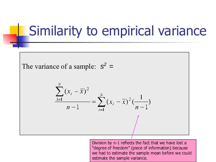
- 59. Similarity to empirical variance The variance of a sample: s2 =
- 60. Symbol Interlude Var(X) = σ2 these symbols are used interchangeably
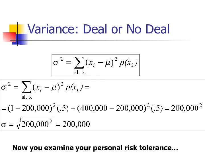
- 61. Variance: Deal or No Deal Now you examine your personal risk tolerance…
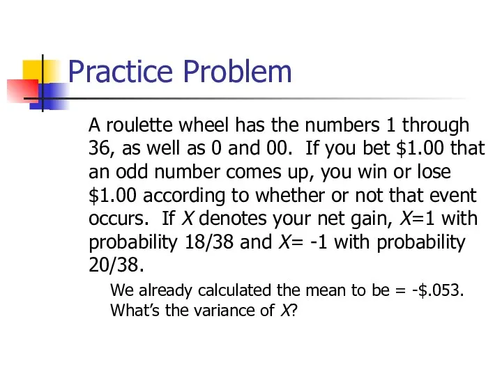
- 62. Practice Problem A roulette wheel has the numbers 1 through 36, as well as 0 and
- 63. Answer Standard deviation is $.99. Interpretation: On average, you’re either 1 dollar above or 1 dollar
- 64. Handy calculation formula! Handy calculation formula (if you ever need to calculate by hand!):
- 65. Var(x) = E(x-μ)2 = E(x2) – [E(x)]2 (your calculation formula!) Proofs (optional!): E(x-μ)2 = E(x2–2μx +
- 66. For example, what’s the variance and standard deviation of the roll of a die?
- 67. **A few notes about Variance as a mathematical operator: If c= a constant number (i.e., not
- 68. Var(c) = 0 Var(c) = 0 Constants don’t vary!
- 69. Var (c+X)= Var(X) Var (c+X)= Var(X) Adding a constant to every instance of a random variable
- 70. Var (c+X)= Var(X) Var (c+X)= Var(X) Adding a constant to every instance of a random variable
- 71. Var(cX)= c2Var(X) Var(cX)= c2Var(X) Multiplying each instance of the random variable by c makes it c-times
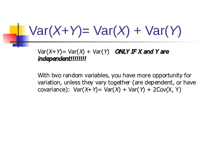
- 72. Var(X+Y)= Var(X) + Var(Y) Var(X+Y)= Var(X) + Var(Y) ONLY IF X and Y are independent!!!!!!!! With
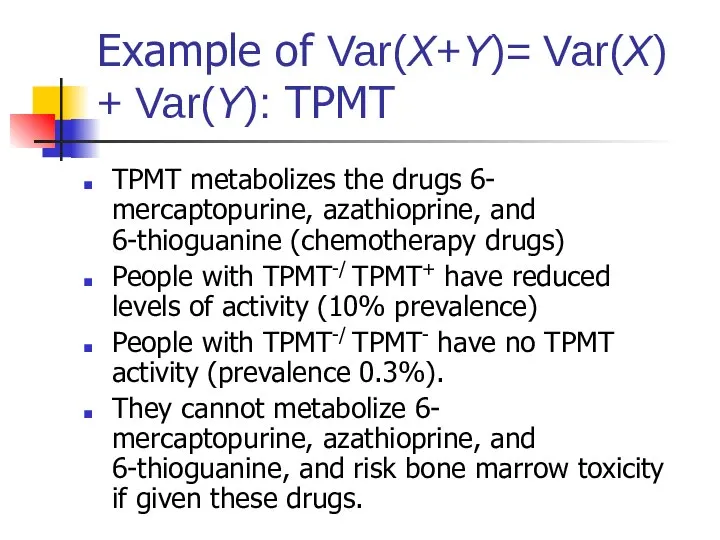
- 73. Example of Var(X+Y)= Var(X) + Var(Y): TPMT TPMT metabolizes the drugs 6- mercaptopurine, azathioprine, and 6-thioguanine
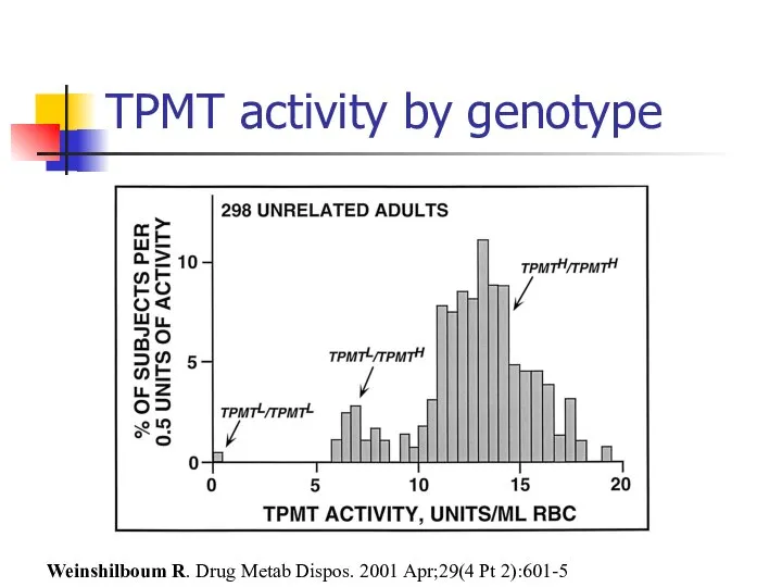
- 74. TPMT activity by genotype Weinshilboum R. Drug Metab Dispos. 2001 Apr;29(4 Pt 2):601-5
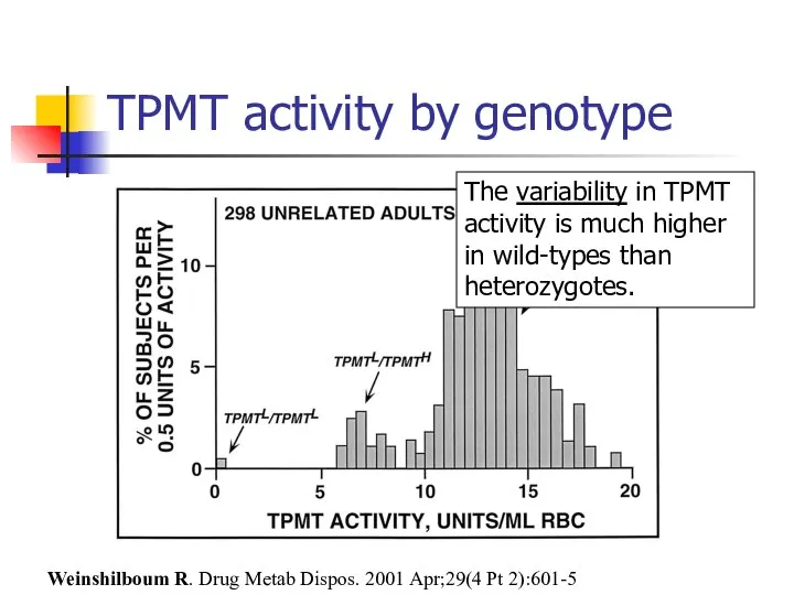
- 75. TPMT activity by genotype Weinshilboum R. Drug Metab Dispos. 2001 Apr;29(4 Pt 2):601-5 The variability in
- 76. TPMT activity by genotype Weinshilboum R. Drug Metab Dispos. 2001 Apr;29(4 Pt 2):601-5 There is variability
- 77. Practice Problem Find the variance and standard deviation for the number of ships to arrive at
- 78. Answer: variance and std dev Interpretation: On an average day, we expect 11.3 ships to arrive
- 79. Practice Problem You toss a coin 100 times. What’s the expected number of heads? What’s the
- 80. Answer: expected value Intuitively, we’d probably all agree that we expect around 50 heads, right? Another
- 81. Answer: variance What’s the variability, though? More tricky. But, again, we could do this for 1
- 82. Or use computer simulation… Flip coins virtually! Flip a virtual coin 100 times; count the number
- 83. Coin tosses… Mean = 50 Std. dev = 5 Follows a normal distribution ∴95% of the
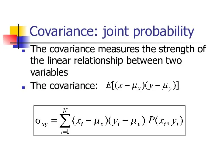
- 84. Covariance: joint probability The covariance measures the strength of the linear relationship between two variables The
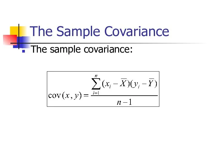
- 85. The Sample Covariance The sample covariance:
- 87. Скачать презентацию
Слайд 3Random variables can be discrete or continuous
Discrete random variables have a countable
Random variables can be discrete or continuous
Discrete random variables have a countable
Слайд 4Probability functions
A probability function maps the possible values of x against their
Probability functions
A probability function maps the possible values of x against their
Слайд 5
Discrete example: roll of a die
Discrete example: roll of a die
Слайд 6Probability mass function (pmf)
Probability mass function (pmf)
Слайд 7Cumulative distribution function (CDF)
Cumulative distribution function (CDF)
Слайд 8Cumulative distribution function
Cumulative distribution function
Слайд 9Examples
1. What’s the probability that you roll a 3 or less?
P(x≤3)=1/2
2.
Examples
1. What’s the probability that you roll a 3 or less?
P(x≤3)=1/2
2.
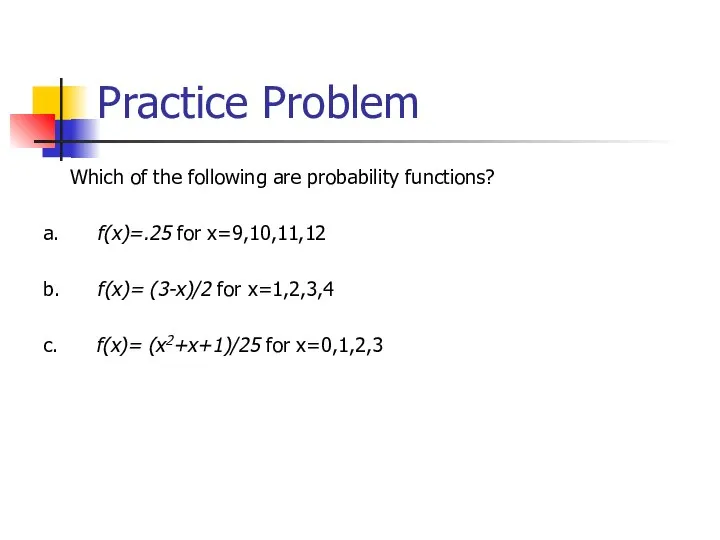
Слайд 10Practice Problem
Which of the following are probability functions?
a. f(x)=.25 for x=9,10,11,12
b. f(x)=
Practice Problem
Which of the following are probability functions?
a. f(x)=.25 for x=9,10,11,12
b. f(x)=
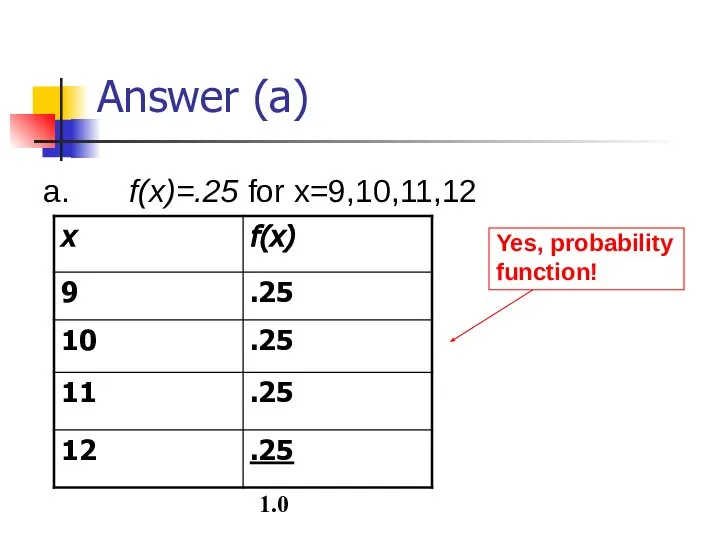
Слайд 11Answer (a)
a. f(x)=.25 for x=9,10,11,12
1.0
Answer (a)
a. f(x)=.25 for x=9,10,11,12
1.0
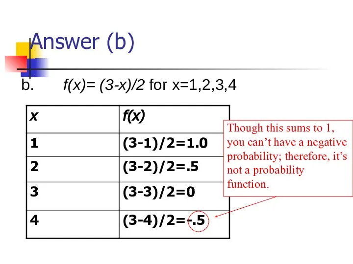
Слайд 12Answer (b)
b. f(x)= (3-x)/2 for x=1,2,3,4
Answer (b)
b. f(x)= (3-x)/2 for x=1,2,3,4
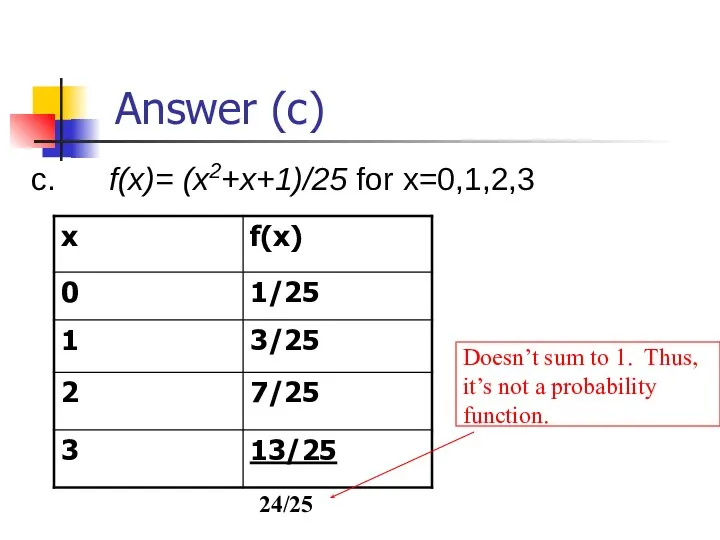
Слайд 13Answer (c)
c. f(x)= (x2+x+1)/25 for x=0,1,2,3
Answer (c)
c. f(x)= (x2+x+1)/25 for x=0,1,2,3
Слайд 14Practice Problem:
The number of ships to arrive at a harbor on any
Practice Problem:
The number of ships to arrive at a harbor on any
Слайд 15Practice Problem:
You are lecturing to a group of 1000 students. You ask
Practice Problem:
You are lecturing to a group of 1000 students. You ask
Слайд 16Important discrete distributions in epidemiology…
Binomial
Yes/no outcomes (dead/alive, treated/untreated, smoker/non-smoker, sick/well, etc.)
Poisson
Counts (e.g.,
Important discrete distributions in epidemiology…
Binomial
Yes/no outcomes (dead/alive, treated/untreated, smoker/non-smoker, sick/well, etc.)
Poisson
Counts (e.g.,
Слайд 17Continuous case
The probability function that accompanies a continuous random variable is a
Continuous case
The probability function that accompanies a continuous random variable is a
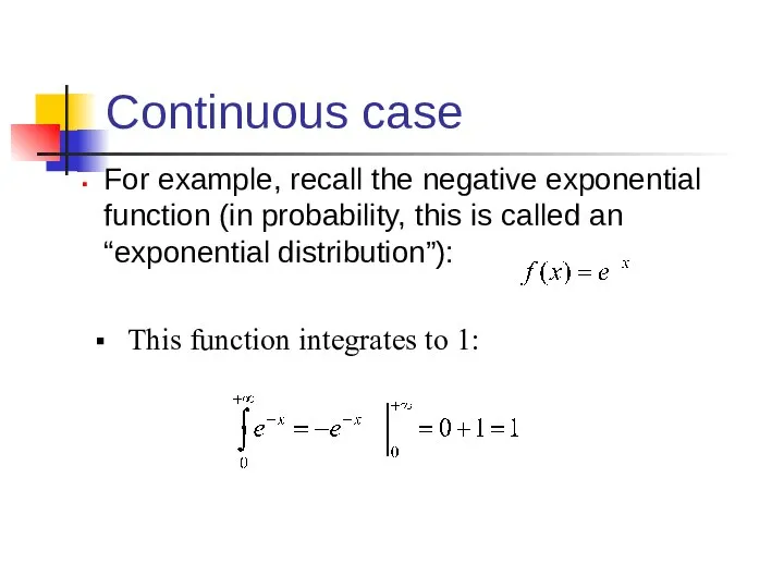
Слайд 18Continuous case
For example, recall the negative exponential function (in probability, this is
Continuous case
For example, recall the negative exponential function (in probability, this is
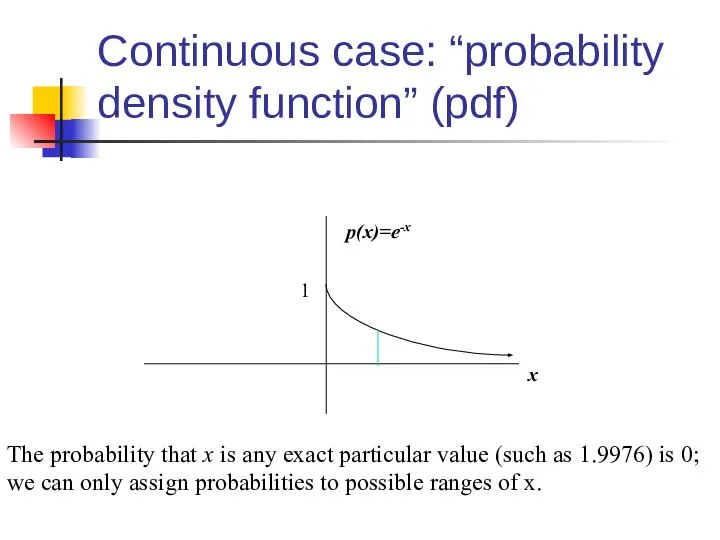
Слайд 19Continuous case: “probability density function” (pdf)
The probability that x is any exact
Continuous case: “probability density function” (pdf)
The probability that x is any exact
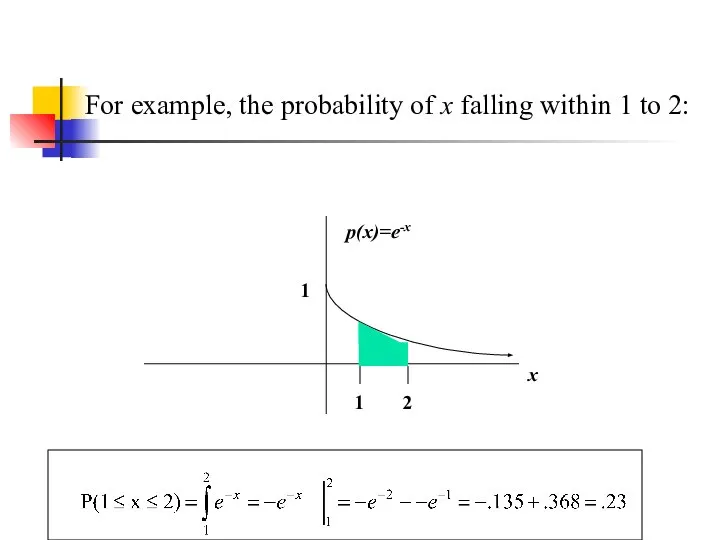
Слайд 20For example, the probability of x falling within 1 to 2:
For example, the probability of x falling within 1 to 2:
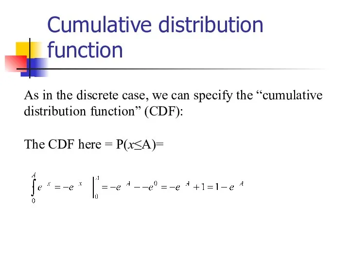
Слайд 21Cumulative distribution function
As in the discrete case, we can specify the “cumulative
Cumulative distribution function
As in the discrete case, we can specify the “cumulative
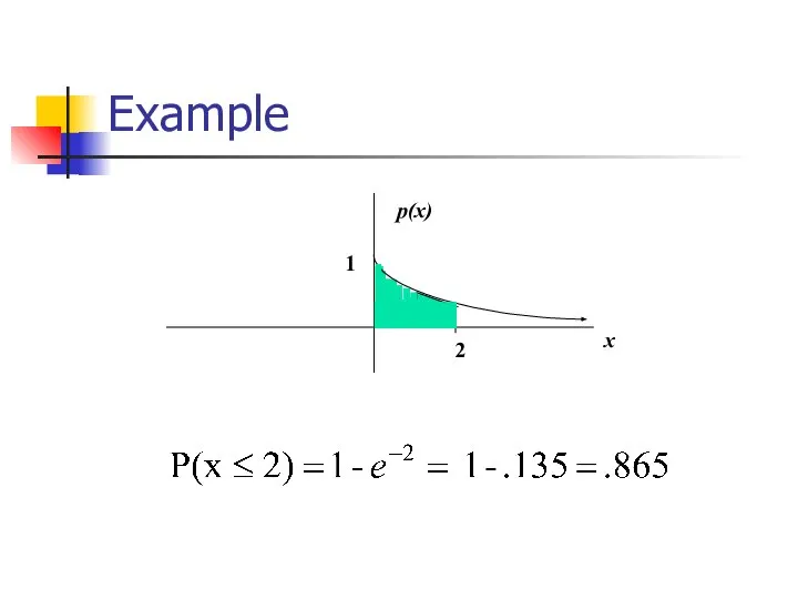
Слайд 22Example
Example
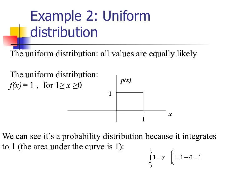
Слайд 23Example 2: Uniform distribution
The uniform distribution: all values are equally likely
The uniform
Example 2: Uniform distribution
The uniform distribution: all values are equally likely
The uniform
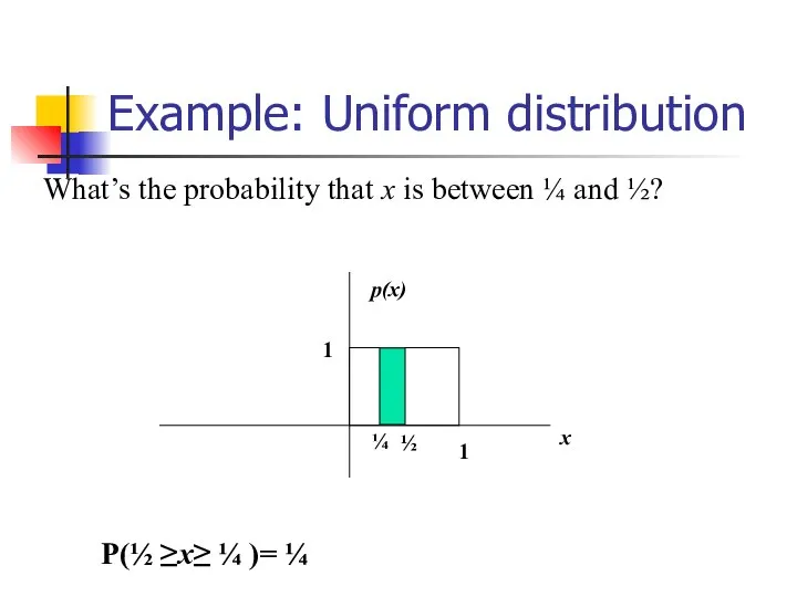
Слайд 24Example: Uniform distribution
What’s the probability that x is between ¼ and ½?
Example: Uniform distribution
What’s the probability that x is between ¼ and ½?
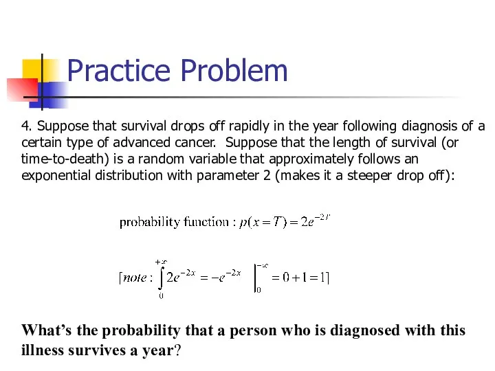
Слайд 25Practice Problem
4. Suppose that survival drops off rapidly in the year
Practice Problem
4. Suppose that survival drops off rapidly in the year
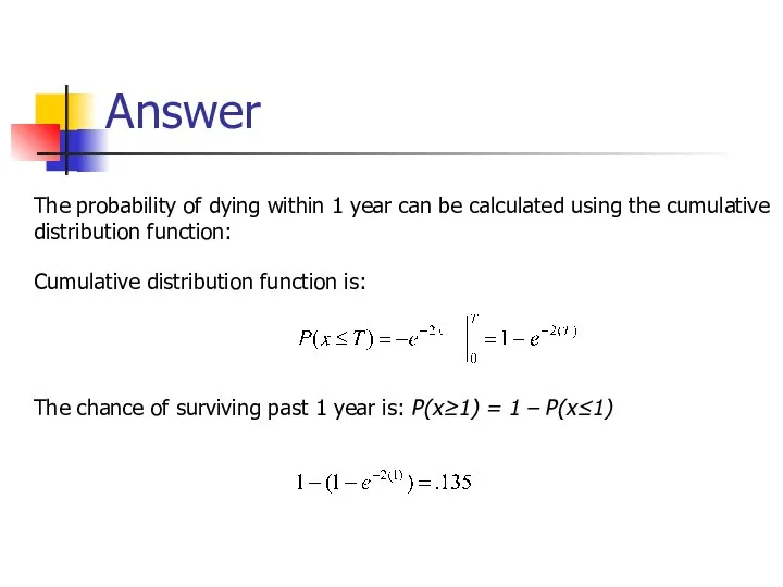
Слайд 26Answer
The probability of dying within 1 year can be calculated using
Answer
The probability of dying within 1 year can be calculated using
Слайд 27Expected Value and Variance
All probability distributions are characterized by an expected value
Expected Value and Variance
All probability distributions are characterized by an expected value
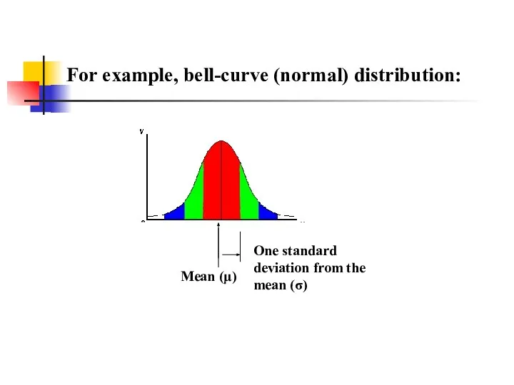
Слайд 28For example, bell-curve (normal) distribution:
For example, bell-curve (normal) distribution:
Слайд 29Expected value, or mean
If we understand the underlying probability function of a
Expected value, or mean
If we understand the underlying probability function of a
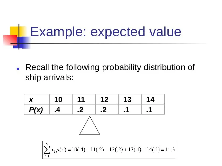
Слайд 30Example: expected value
Recall the following probability distribution of ship arrivals:
Example: expected value
Recall the following probability distribution of ship arrivals:
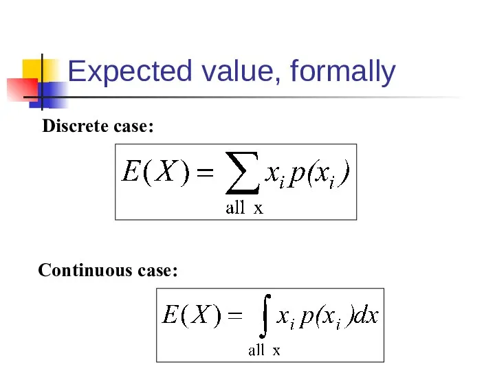
Слайд 31Expected value, formally
Discrete case:
Continuous case:
Expected value, formally
Discrete case:
Continuous case:

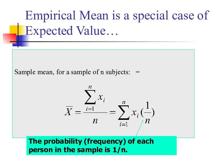
Слайд 32Empirical Mean is a special case of Expected Value…
Sample mean, for a
Empirical Mean is a special case of Expected Value…
Sample mean, for a
Слайд 33Expected value, formally
Discrete case:
Continuous case:
Expected value, formally
Discrete case:
Continuous case:
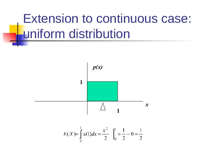
Слайд 34Extension to continuous case:
uniform distribution
x
p(x)
1
1
Extension to continuous case:
uniform distribution
x
p(x)
1
1
Слайд 35Symbol Interlude
E(X) = µ
these symbols are used interchangeably
Symbol Interlude
E(X) = µ
these symbols are used interchangeably
Слайд 36Expected Value
Expected value is an extremely useful concept for good decision-making!
Expected Value
Expected value is an extremely useful concept for good decision-making!
Слайд 37Example: the lottery
The Lottery (also known as a tax on people who
Example: the lottery
The Lottery (also known as a tax on people who
Слайд 38Lottery
Calculate the probability of winning in 1 try:
The probability function (note, sums
Lottery
Calculate the probability of winning in 1 try:
The probability function (note, sums
Слайд 39Expected Value
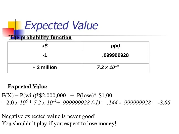
The probability function
Expected Value
E(X) = P(win)*$2,000,000 + P(lose)*-$1.00
= 2.0 x
Expected Value
The probability function
Expected Value
E(X) = P(win)*$2,000,000 + P(lose)*-$1.00
= 2.0 x
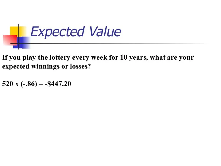
Слайд 40Expected Value
If you play the lottery every week for 10 years, what
Expected Value
If you play the lottery every week for 10 years, what
Слайд 41
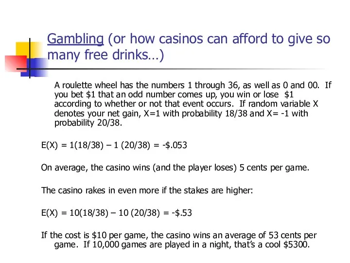
Gambling (or how casinos can afford to give so many free drinks…)
A
Gambling (or how casinos can afford to give so many free drinks…)
A
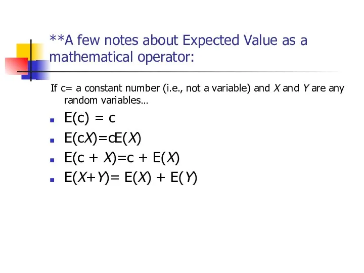
Слайд 42**A few notes about Expected Value as a mathematical operator:
If c= a
**A few notes about Expected Value as a mathematical operator:
If c= a
Слайд 43
E(c) = c
E(c) = c
Example: If you cash in soda
E(c) = c
E(c) = c
Example: If you cash in soda
Слайд 44E(cX)=cE(X)
E(cX)=cE(X)
Example: If the casino charges $10 per game instead of $1, then
E(cX)=cE(X)
E(cX)=cE(X)
Example: If the casino charges $10 per game instead of $1, then
Слайд 45E(c + X)=c + E(X)
E(c + X)=c + E(X)
Example, if the casino
E(c + X)=c + E(X)
E(c + X)=c + E(X)
Example, if the casino
Слайд 46E(X+Y)= E(X) + E(Y)
E(X+Y)= E(X) + E(Y)
Example: If you play
E(X+Y)= E(X) + E(Y)
E(X+Y)= E(X) + E(Y)
Example: If you play
Слайд 47Practice Problem
If a disease is fairly rare and the antibody test is
Practice Problem
If a disease is fairly rare and the antibody test is
Слайд 48Answer (a)
a. Suppose a particular disease has a prevalence of 10% in
Answer (a)
a. Suppose a particular disease has a prevalence of 10% in
Слайд 49Answer (b)
b. What if you pool only 10 samples at a
Answer (b)
b. What if you pool only 10 samples at a
Слайд 50Answer (c)
c. 5 samples at a time?
E(X) = (.90)5 (1) + [1-.905]
Answer (c)
c. 5 samples at a time?
E(X) = (.90)5 (1) + [1-.905]
Слайд 51Practice Problem
If X is a random integer between 1 and
Practice Problem
If X is a random integer between 1 and
Слайд 52Answer
If X is a random integer between 1 and 10, what’s the
Answer
If X is a random integer between 1 and 10, what’s the
Слайд 53Expected value isn’t everything though…
Take the show “Deal or No Deal”
Everyone know
Expected value isn’t everything though…
Take the show “Deal or No Deal”
Everyone know
Слайд 54Deal or No Deal…
This could really be represented as a probability distribution
Deal or No Deal…
This could really be represented as a probability distribution
Слайд 55Expected value doesn’t help…
Expected value doesn’t help…
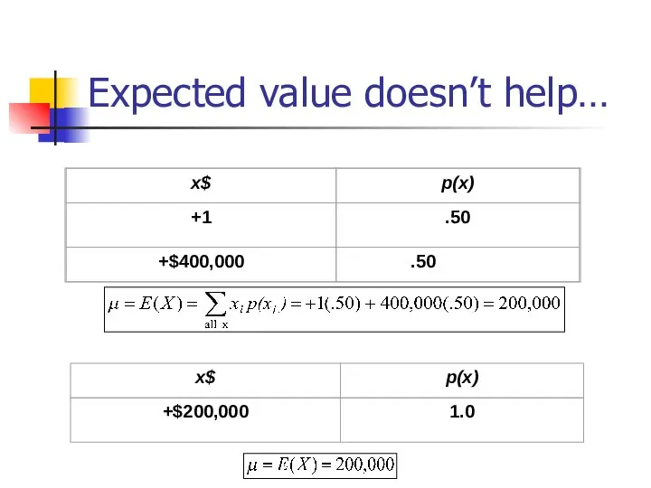
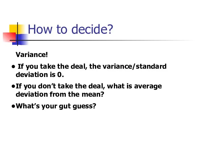
Слайд 56How to decide?
Variance!
If you take the deal, the variance/standard deviation
How to decide?
Variance!
If you take the deal, the variance/standard deviation
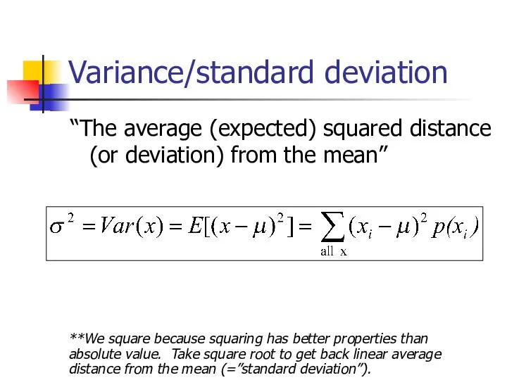
Слайд 57Variance/standard deviation
“The average (expected) squared distance (or deviation) from the mean”
**We square
Variance/standard deviation
“The average (expected) squared distance (or deviation) from the mean”
**We square
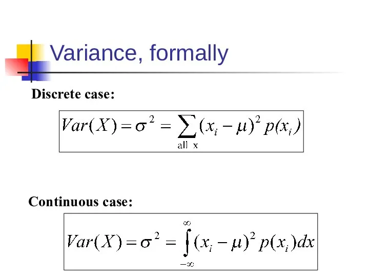
Слайд 58Variance, formally
Discrete case:
Continuous case:
Variance, formally
Discrete case:
Continuous case:
Слайд 59Similarity to empirical variance
The variance of a sample: s2 =
Similarity to empirical variance
The variance of a sample: s2 =
Слайд 60Symbol Interlude
Var(X) = σ2
these symbols are used interchangeably
Symbol Interlude
Var(X) = σ2
these symbols are used interchangeably
Слайд 61Variance: Deal or No Deal
Now you examine your personal risk tolerance…
Variance: Deal or No Deal
Now you examine your personal risk tolerance…
Слайд 62Practice Problem
A roulette wheel has the numbers 1 through 36, as well
Practice Problem
A roulette wheel has the numbers 1 through 36, as well
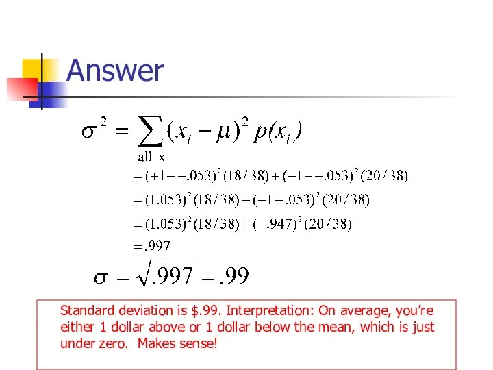
Слайд 63Answer
Standard deviation is $.99. Interpretation: On average, you’re either 1 dollar above
Answer
Standard deviation is $.99. Interpretation: On average, you’re either 1 dollar above
Слайд 64Handy calculation formula!
Handy calculation formula (if you ever need to calculate by
Handy calculation formula!
Handy calculation formula (if you ever need to calculate by
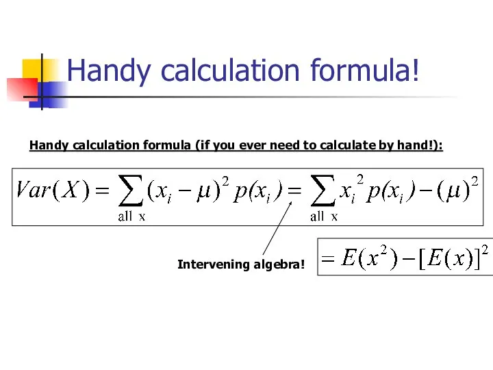
Слайд 65Var(x) = E(x-μ)2 = E(x2) – [E(x)]2 (your calculation formula!)
Proofs (optional!):
E(x-μ)2
Var(x) = E(x-μ)2 = E(x2) – [E(x)]2 (your calculation formula!)
Proofs (optional!):
E(x-μ)2
![Var(x) = E(x-μ)2 = E(x2) – [E(x)]2 (your calculation formula!) Proofs (optional!):](/_ipx/f_webp&q_80&fit_contain&s_1440x1080/imagesDir/jpg/1058868/slide-64.jpg)
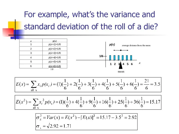
Слайд 66For example, what’s the variance and standard deviation of the roll of
For example, what’s the variance and standard deviation of the roll of
Слайд 67**A few notes about Variance as a mathematical operator:
If c= a constant
**A few notes about Variance as a mathematical operator:
If c= a constant
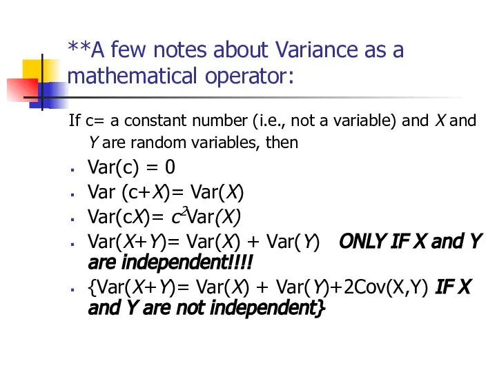
Слайд 68Var(c) = 0
Var(c) = 0
Constants don’t vary!
Var(c) = 0
Var(c) = 0
Constants don’t vary!
Слайд 69Var (c+X)= Var(X)
Var (c+X)= Var(X)
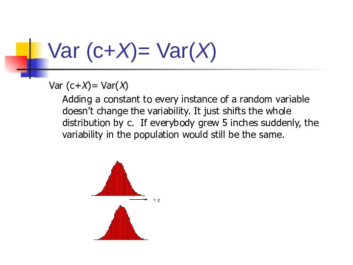
Adding a constant to every instance of a
Var (c+X)= Var(X)
Var (c+X)= Var(X)
Adding a constant to every instance of a
Слайд 70Var (c+X)= Var(X)
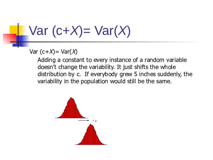
Var (c+X)= Var(X)
Adding a constant to every instance of a
Var (c+X)= Var(X)
Var (c+X)= Var(X)
Adding a constant to every instance of a
Слайд 71Var(cX)= c2Var(X)
Var(cX)= c2Var(X)
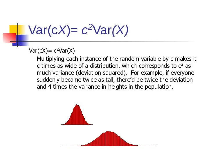
Multiplying each instance of the random variable by c makes
Var(cX)= c2Var(X)
Var(cX)= c2Var(X)
Multiplying each instance of the random variable by c makes
Слайд 72Var(X+Y)= Var(X) + Var(Y)
Var(X+Y)= Var(X) + Var(Y) ONLY IF X and Y
Var(X+Y)= Var(X) + Var(Y)
Var(X+Y)= Var(X) + Var(Y) ONLY IF X and Y
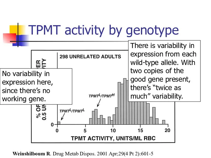
Слайд 73Example of Var(X+Y)= Var(X) + Var(Y): TPMT
TPMT metabolizes the drugs 6- mercaptopurine,
Example of Var(X+Y)= Var(X) + Var(Y): TPMT
TPMT metabolizes the drugs 6- mercaptopurine,
Слайд 74TPMT activity by genotype
Weinshilboum R. Drug Metab Dispos. 2001 Apr;29(4 Pt 2):601-5
TPMT activity by genotype
Weinshilboum R. Drug Metab Dispos. 2001 Apr;29(4 Pt 2):601-5
Слайд 75TPMT activity by genotype
Weinshilboum R. Drug Metab Dispos. 2001 Apr;29(4 Pt 2):601-5
The
TPMT activity by genotype
Weinshilboum R. Drug Metab Dispos. 2001 Apr;29(4 Pt 2):601-5
The
Слайд 76TPMT activity by genotype
Weinshilboum R. Drug Metab Dispos. 2001 Apr;29(4 Pt 2):601-5
There
TPMT activity by genotype
Weinshilboum R. Drug Metab Dispos. 2001 Apr;29(4 Pt 2):601-5
There
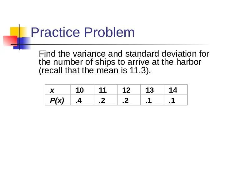
Слайд 77Practice Problem
Find the variance and standard deviation for the number of ships
Practice Problem
Find the variance and standard deviation for the number of ships
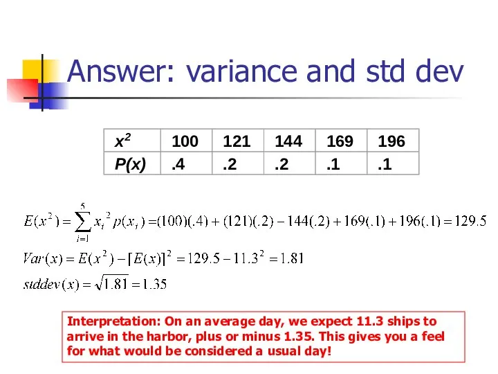
Слайд 78Answer: variance and std dev
Interpretation: On an average day, we expect 11.3
Answer: variance and std dev
Interpretation: On an average day, we expect 11.3
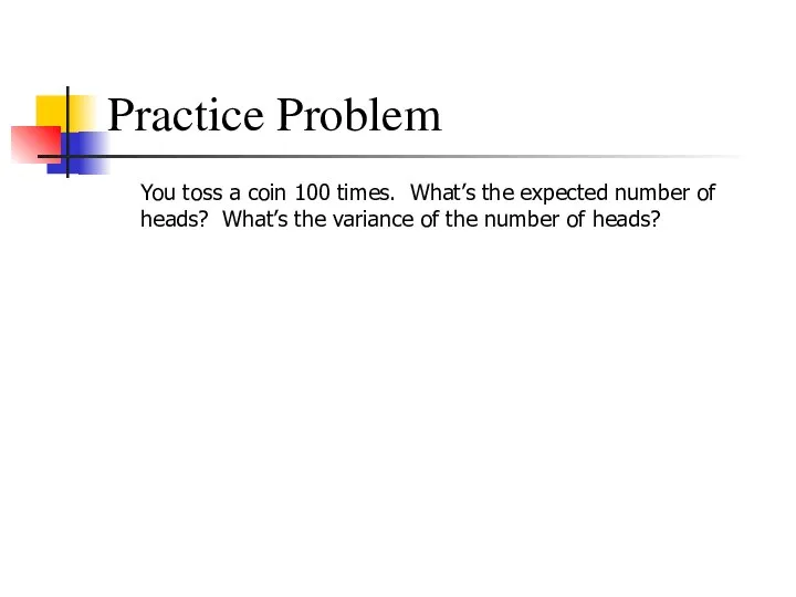
Слайд 79Practice Problem
You toss a coin 100 times. What’s the expected number of
Practice Problem
You toss a coin 100 times. What’s the expected number of
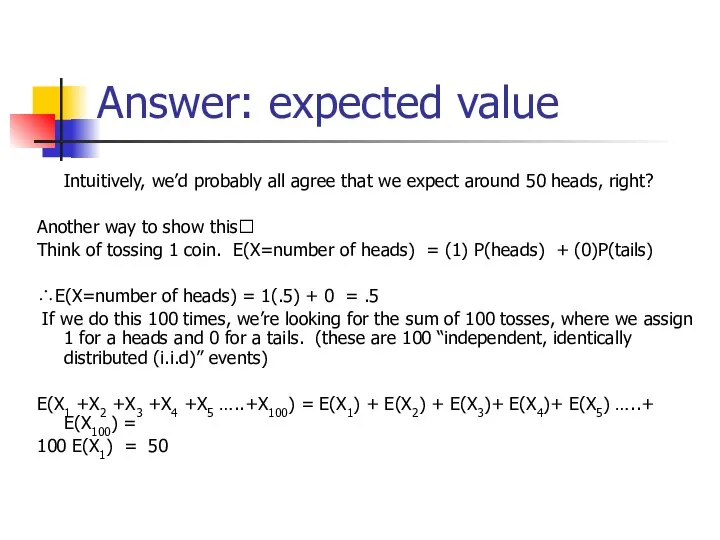
Слайд 80Answer: expected value
Intuitively, we’d probably all agree that we expect around 50
Answer: expected value
Intuitively, we’d probably all agree that we expect around 50
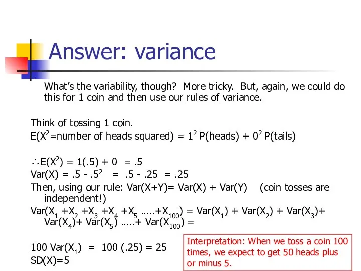
Слайд 81Answer: variance
What’s the variability, though? More tricky. But, again, we could do
Answer: variance
What’s the variability, though? More tricky. But, again, we could do
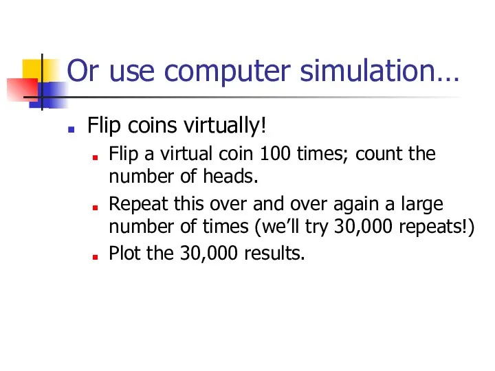
Слайд 82Or use computer simulation…
Flip coins virtually!
Flip a virtual coin 100 times; count
Or use computer simulation…
Flip coins virtually!
Flip a virtual coin 100 times; count
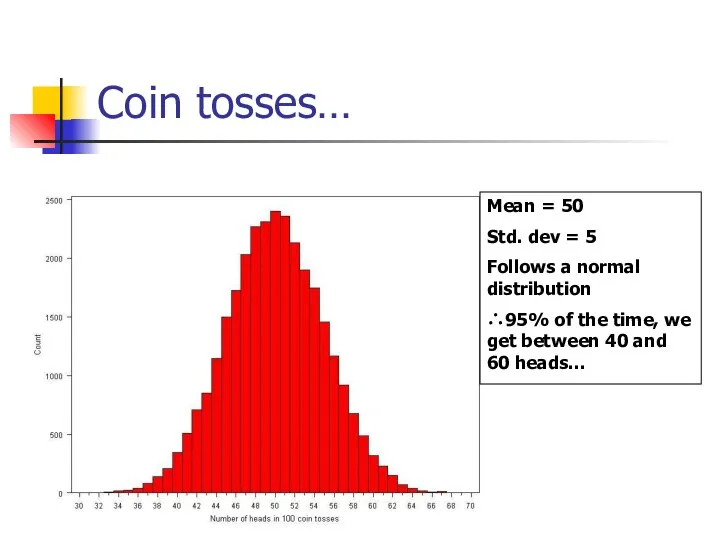
Слайд 83Coin tosses…
Mean = 50
Std. dev = 5
Follows a normal distribution
∴95% of the
Coin tosses…
Mean = 50
Std. dev = 5
Follows a normal distribution
∴95% of the
Слайд 84Covariance: joint probability
The covariance measures the strength of the linear relationship between
Covariance: joint probability
The covariance measures the strength of the linear relationship between
Слайд 85The Sample Covariance
The sample covariance:
The Sample Covariance
The sample covariance:
 Тренажёр. Табличное умножение. В сказочном лесу
 Решение практико-ориентированных задач ОГЭ 2021г. Задачи про шины
 Действия с величинами. Урок №4
 Population statistical methods
 Концентрация кислоты
 Алгебра. Число. Уравнение. Тождество. Функция
 Преобразование графиков квадратичной функции. 8 класс
 Обыкновенные дроби
 Числа от 11 до 20. Нумерация
 Урок–путешествие в страну Дроби
 Теорема Пифагора. Решение задач
 Алгоритмы и структуры данных. Семестр 2. Лекция 1. Графы. 07.09
 Разработка обучающей программы по нахождению элементов треугольника
 Презентация на тему Итоговое повторение по темам "Окружность", "Многоугольники"
  Математический проект
 Параллельные плоскости. Признак параллельности двух плоскостей
 Устный счет в пределах 10
 Симметрия вокруг нас
 Решение задач с помощью составления систем уравнений
 Математический диктант. 6 класс
 Окружность. Вписанные углы
 Правильный многогранник
 Дифференциальные уравнения
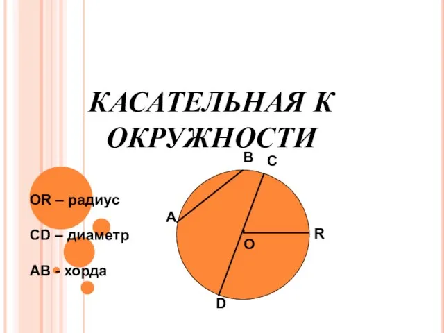 08.09
08.09 Презентация на тему Решение задач на применение свойств подобия
  Учимся считать. Интерактивный тренажёр
 Построение графика квадратичной функции у=ах2+bx+c, a не равно 0
 Некоторые свойства прямоугольных треугольников. Решение задач