- Descriptive Statistics Graphing Techniques

Содержание
- 2. Points and grades from examination
- 3. Sample size n=30 Data sorting → Frequency table both for quantitative and qualitative data
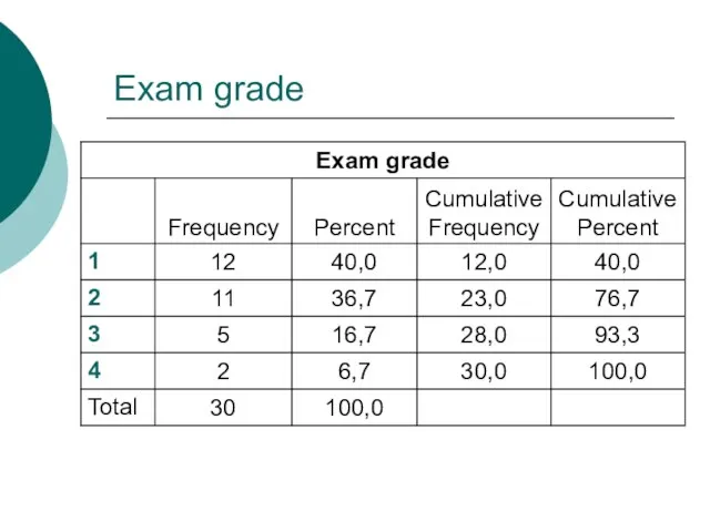
- 4. Exam grade
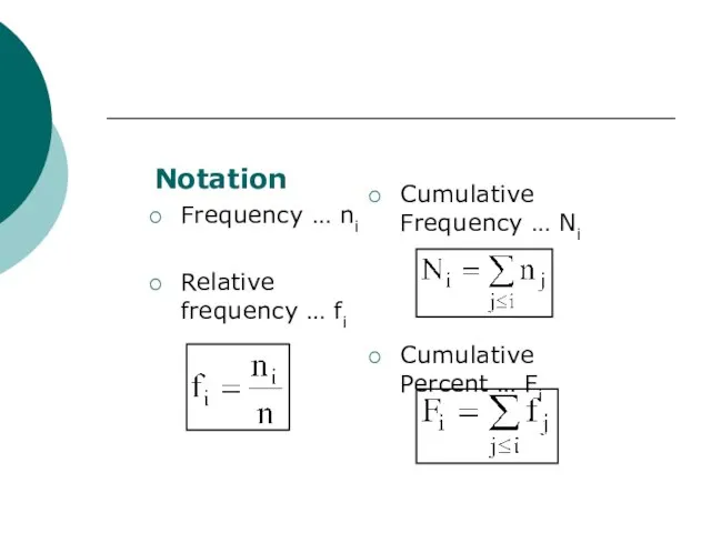
- 5. Notation Frequency … ni Relative frequency … fi Cumulative Frequency … Ni Cumulative Percent … Fi
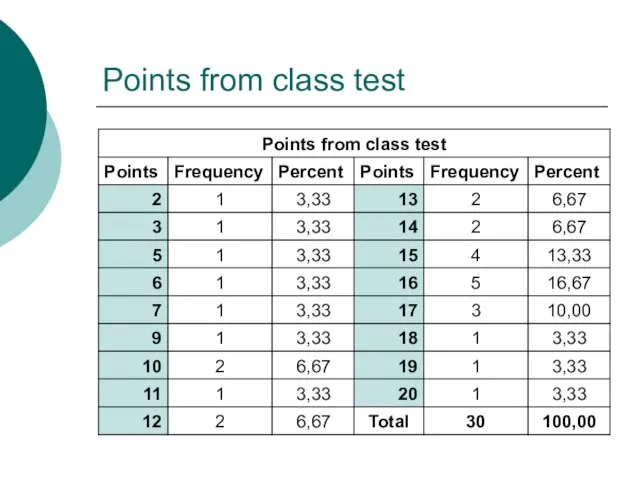
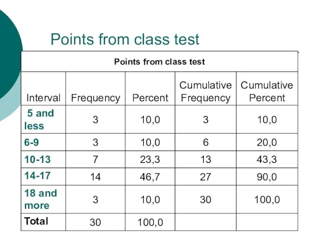
- 6. Points from class test
- 7. Quantitative variables Grouping into class intervals
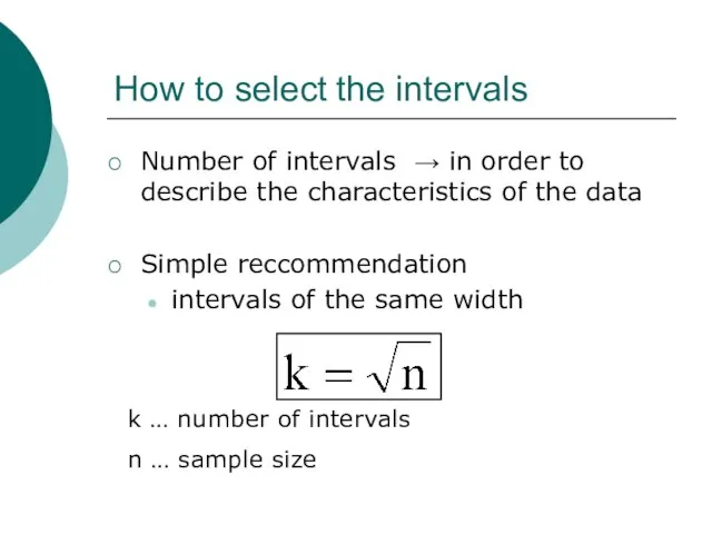
- 8. How to select the intervals Number of intervals → in order to describe the characteristics of
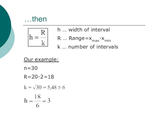
- 9. …then h … width of interval R … Range=xmax-xmin k … number of intervals Our example:
- 10. Points from class test
- 11. Measures of Central Tendency Measures that represent with a proper value the tendency of most data
- 12. The arithmetic mean Notation arithmetic mean …… the sum of the values of a variable divided
- 13. Properties of the arithmetic mean it is expressed in the same unit of measure as the
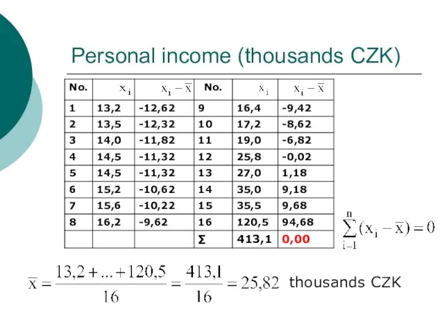
- 14. Personal income (thousands CZK) thousands CZK
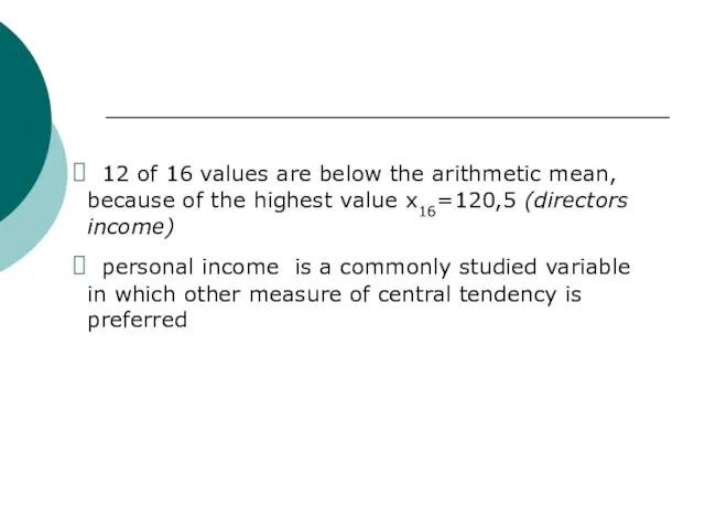
- 15. 12 of 16 values are below the arithmetic mean, because of the highest value x16=120,5 (directors
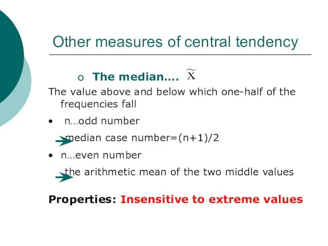
- 16. Other measures of central tendency The median…. The value above and below which one-half of the
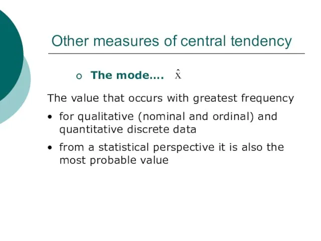
- 17. Other measures of central tendency The mode…. The value that occurs with greatest frequency for qualitative
- 18. Personal income (thousands CZK) n=16… even number the median the mode
- 19. Personal income (thousands CZK) n=16… even number the median the mode
- 20. Use of mean, median and mode The arithmetic mean member of mathematical system in advanced statistical
- 21. The mean, median, mode and skewness
- 22. to describe the spread of the data, its variation around a central value we want to
- 24. The Range….R it is the distance between the largest and the smallest value R=xmax-xmin it does
- 25. The Variance…s2 it is an average squared deviation of each value from the mean it is
- 26. Working formulas For easier computation Formula 1 Formula 2
- 27. the variance explains both the variability of the values around the arithmetic mean the variability among
- 28. The Standard Deviation…s it is the square root of variance when computing the variation based on
- 29. it is expressed in the same unit of measure as the observed variable the size of
- 30. Two data sets with the same arithmetic mean and different SD
- 31. Example – Personal income (thousands CZK) thousands CZK
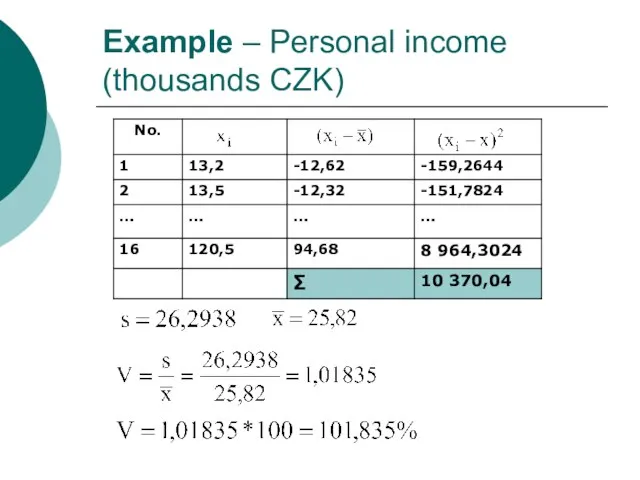
- 32. Coefficient of Variation…V the ratio of the standard deviation to the mean often reported as a
- 33. it is a relative measure of dispersion used when comparing two data sets with different units
- 34. Example – Personal income (thousands CZK)
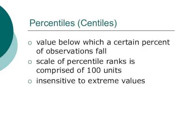
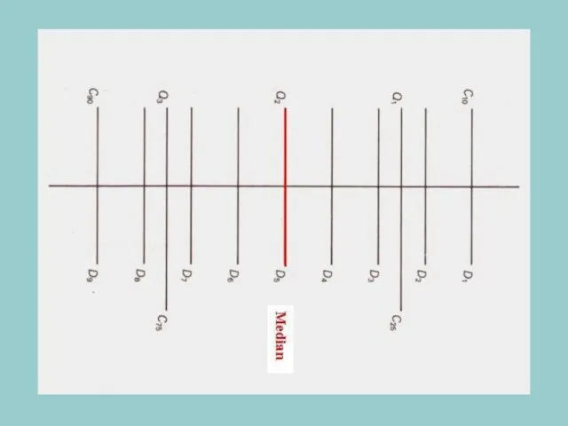
- 35. Percentiles (Centiles) value below which a certain percent of observations fall scale of percentile ranks is
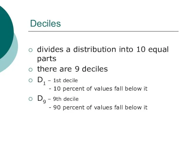
- 36. Deciles divides a distribution into 10 equal parts there are 9 deciles D1 – 1st decile
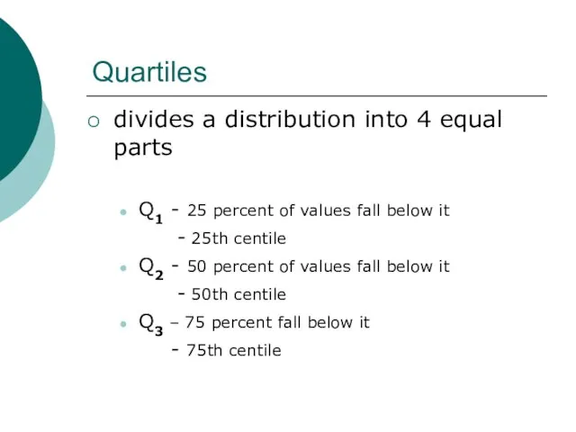
- 37. divides a distribution into 4 equal parts Q1 - 25 percent of values fall below it
- 39. Graphing Techniques
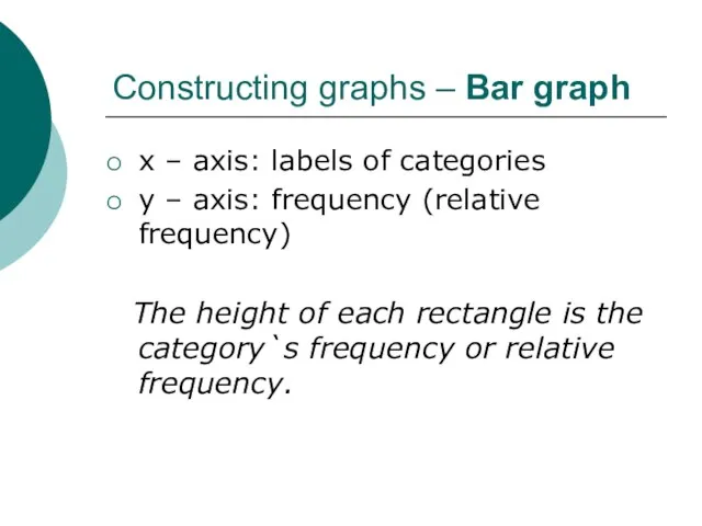
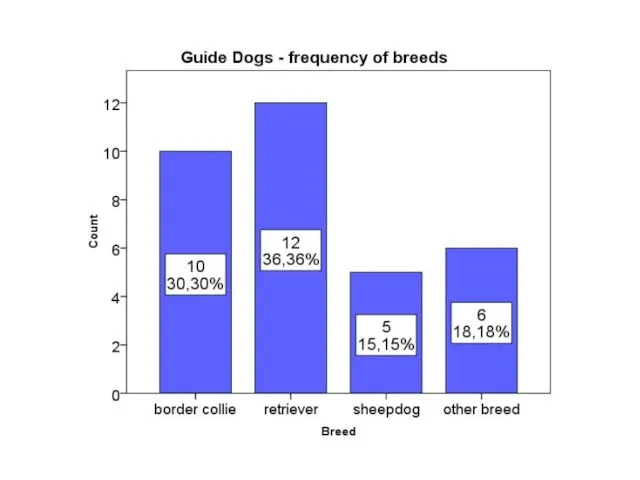
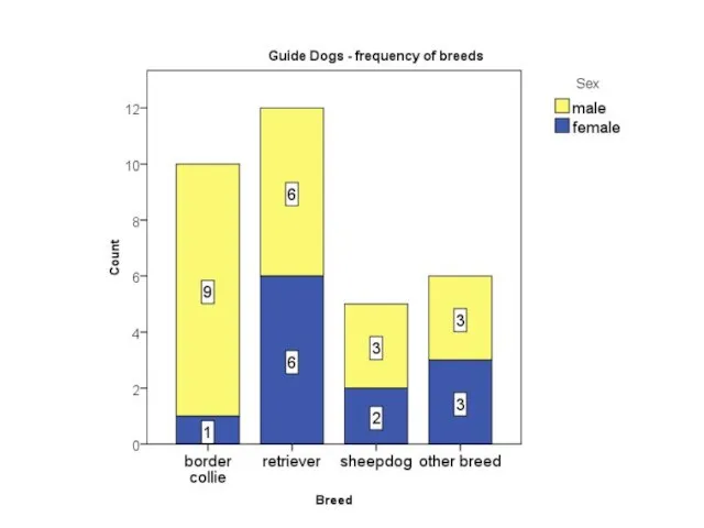
- 40. Constructing graphs – Bar graph x – axis: labels of categories y – axis: frequency (relative
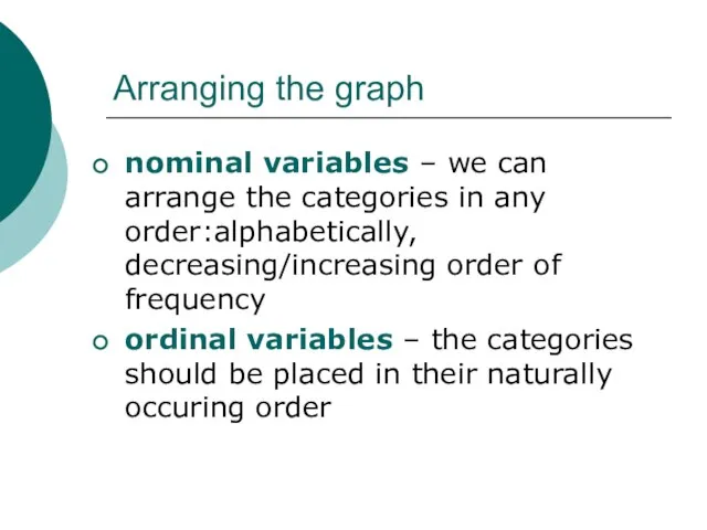
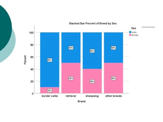
- 41. Arranging the graph nominal variables – we can arrange the categories in any order:alphabetically, decreasing/increasing order
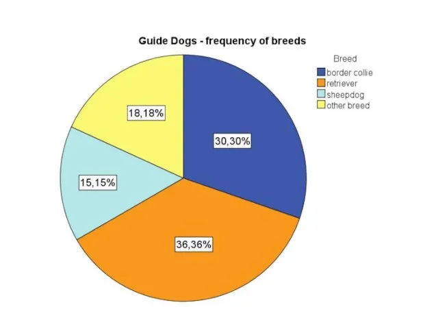
- 45. Constructing graphs – Pie graph Pie chart – a circle divided into sectors each sector represents
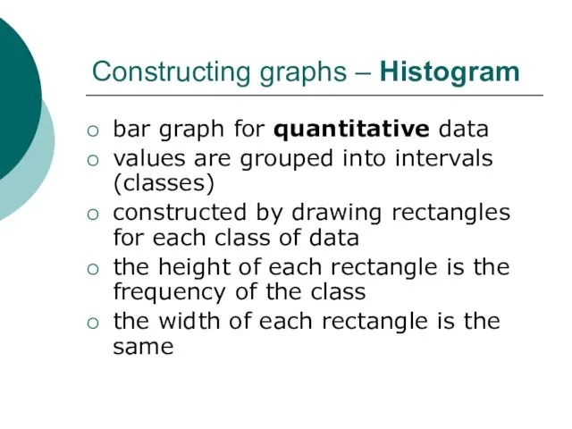
- 47. Constructing graphs – Histogram bar graph for quantitative data values are grouped into intervals (classes) constructed
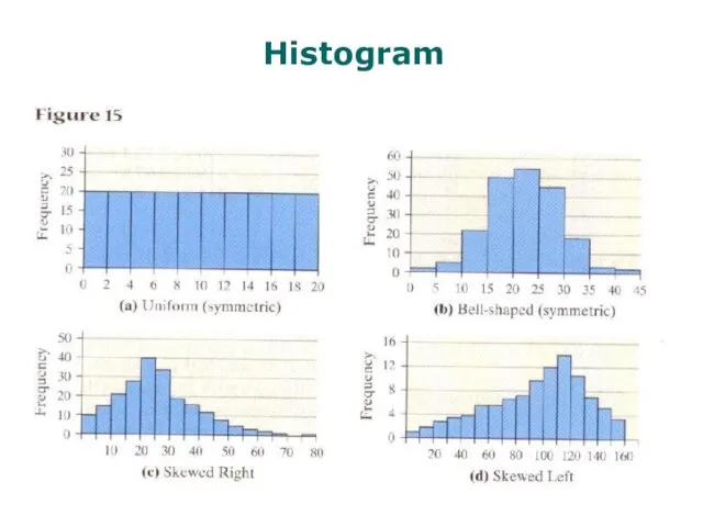
- 49. Histogram
- 51. Constructing graphs – Boxplot box-and-whisker diagram five number summary
- 52. Boxplot Q3 Q1 Q2
- 55. Скачать презентацию
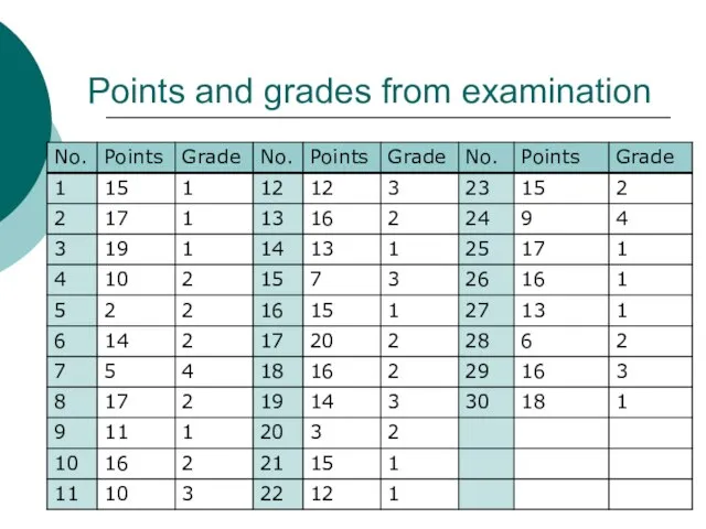
Слайд 3Sample size n=30
Data sorting → Frequency table
both for quantitative and qualitative data
Sample size n=30
Data sorting → Frequency table
both for quantitative and qualitative data
Слайд 4Exam grade
Exam grade
Слайд 5Notation
Frequency … ni
Relative frequency … fi
Cumulative Frequency … Ni
Cumulative Percent … Fi
Notation
Frequency … ni
Relative frequency … fi
Cumulative Frequency … Ni
Cumulative Percent … Fi
Слайд 6Points from class test
Points from class test
Слайд 7Quantitative variables
Grouping into class intervals
Quantitative variables
Grouping into class intervals
Слайд 8How to select the intervals
Number of intervals → in order to describe
How to select the intervals
Number of intervals → in order to describe
Слайд 9…then
h … width of interval
R … Range=xmax-xmin
k … number of intervals
Our example:
n=30
R=20-2=18
…then
h … width of interval
R … Range=xmax-xmin
k … number of intervals
Our example:
n=30
R=20-2=18
Слайд 10Points from class test
Points from class test
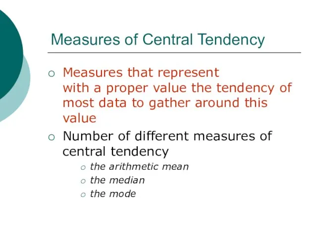
Слайд 11Measures of Central Tendency
Measures that represent
with a proper value the tendency
Measures of Central Tendency
Measures that represent with a proper value the tendency
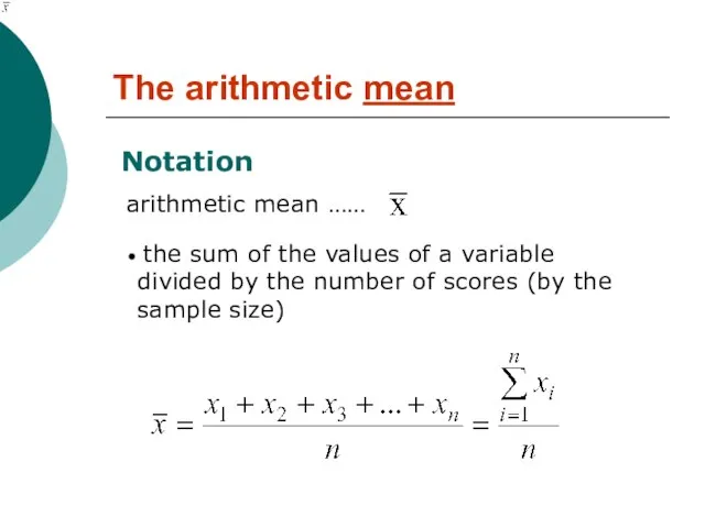
Слайд 12The arithmetic mean
Notation
arithmetic mean ……
the sum of the values of a
The arithmetic mean
Notation
arithmetic mean ……
the sum of the values of a
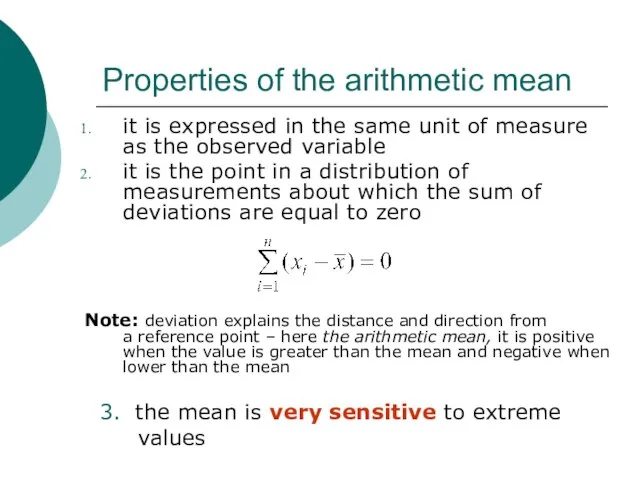
Слайд 13Properties of the arithmetic mean
it is expressed in the same unit of
Properties of the arithmetic mean
it is expressed in the same unit of
Слайд 14Personal income (thousands CZK)
thousands CZK
Personal income (thousands CZK)
thousands CZK
Слайд 15 12 of 16 values are below the arithmetic mean, because of
12 of 16 values are below the arithmetic mean, because of
Слайд 16Other measures of central tendency
The median….
The value above and below which one-half
Other measures of central tendency
The median….
The value above and below which one-half
Слайд 17Other measures of central tendency
The mode….
The value that occurs with greatest frequency
for
Other measures of central tendency
The mode….
The value that occurs with greatest frequency
for
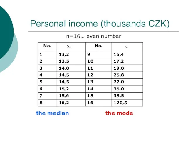
Слайд 18Personal income (thousands CZK)
n=16… even number
the median the mode
Personal income (thousands CZK)
n=16… even number
the median the mode
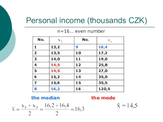
Слайд 19Personal income (thousands CZK)
n=16… even number
the median the mode
Personal income (thousands CZK)
n=16… even number
the median the mode
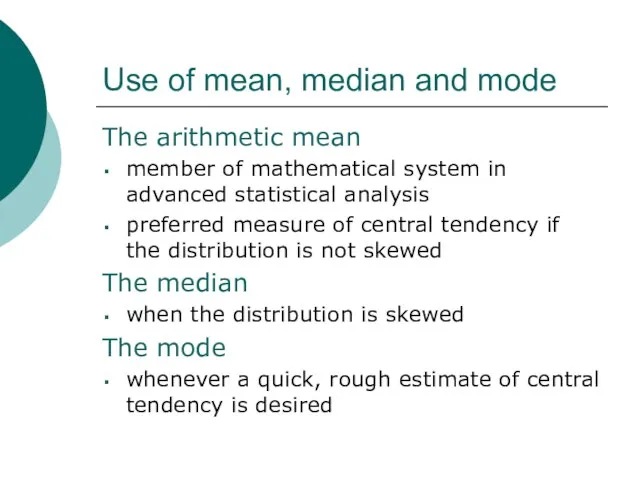
Слайд 20Use of mean, median and mode
The arithmetic mean
member of mathematical system in
Use of mean, median and mode
The arithmetic mean
member of mathematical system in
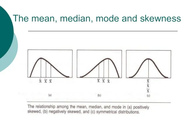
Слайд 21The mean, median, mode and skewness
The mean, median, mode and skewness
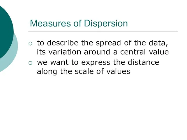
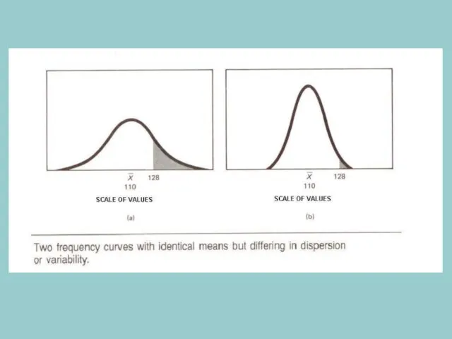
Слайд 22to describe the spread of the data, its variation around a central
to describe the spread of the data, its variation around a central
Слайд 24The Range….R
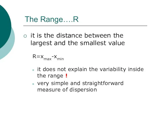
it is the distance between the largest and the smallest value
R=xmax-xmin
it
The Range….R
it is the distance between the largest and the smallest value
R=xmax-xmin
it
Слайд 25The Variance…s2
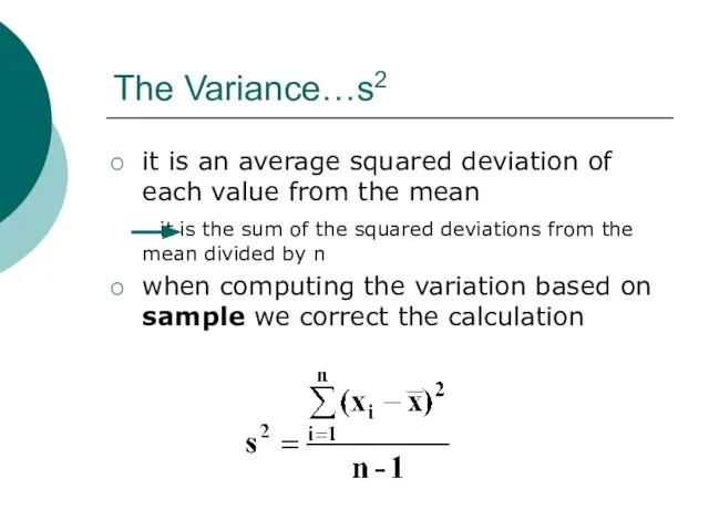
it is an average squared deviation of each value from the
The Variance…s2
it is an average squared deviation of each value from the
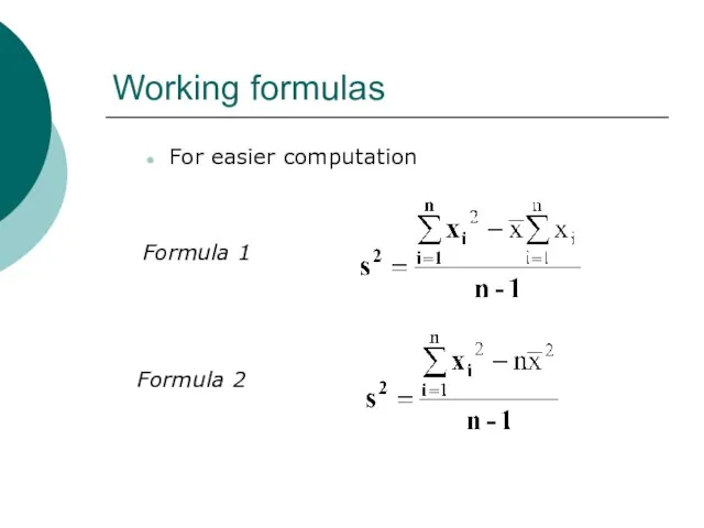
Слайд 26Working formulas
For easier computation
Formula 1
Formula 2
Working formulas
For easier computation
Formula 1
Formula 2
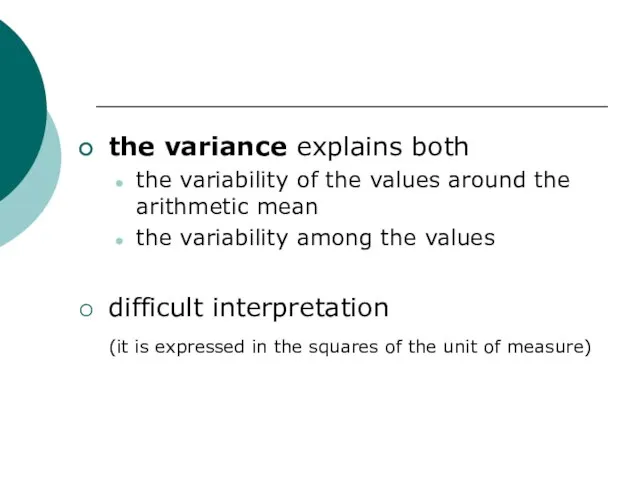
Слайд 27the variance explains both
the variability of the values around the arithmetic
the variance explains both
the variability of the values around the arithmetic
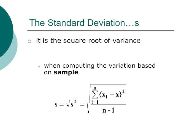
Слайд 28The Standard Deviation…s
it is the square root of variance
when computing the variation
The Standard Deviation…s
it is the square root of variance
when computing the variation
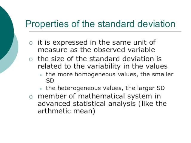
Слайд 29it is expressed in the same unit of measure as the observed
it is expressed in the same unit of measure as the observed
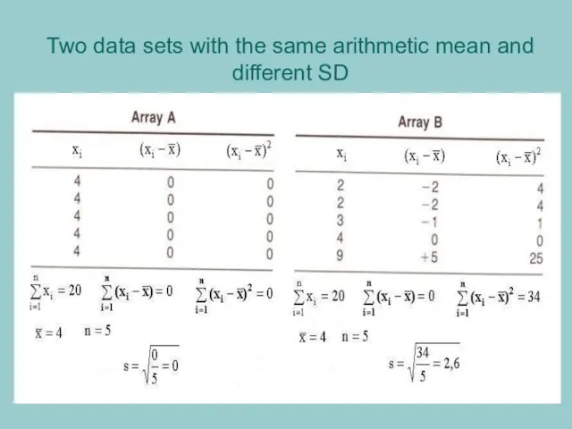
Слайд 30Two data sets with the same arithmetic mean and different SD
Two data sets with the same arithmetic mean and different SD
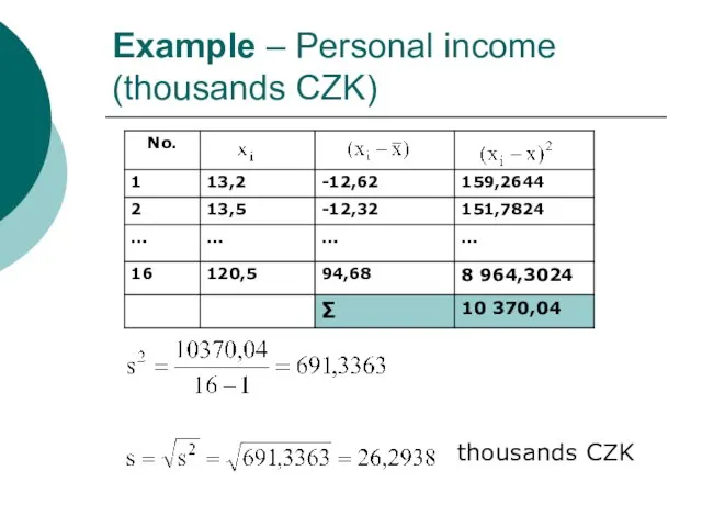
Слайд 31Example – Personal income (thousands CZK)
thousands CZK
Example – Personal income (thousands CZK)
thousands CZK
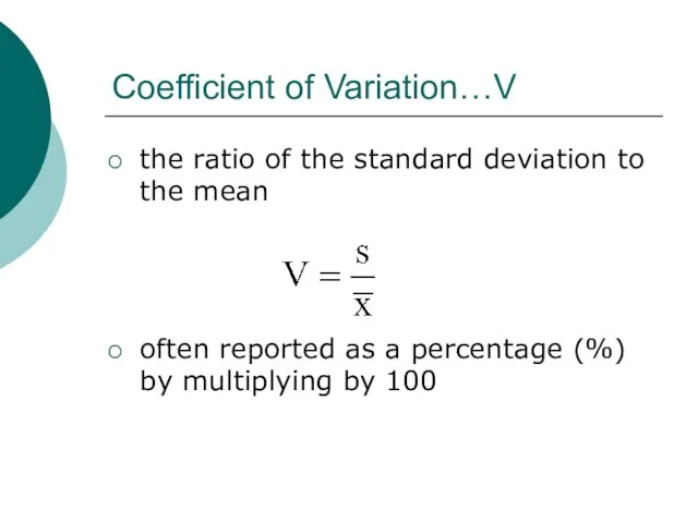
Слайд 32Coefficient of Variation…V
the ratio of the standard deviation to the mean
often reported
Coefficient of Variation…V
the ratio of the standard deviation to the mean
often reported
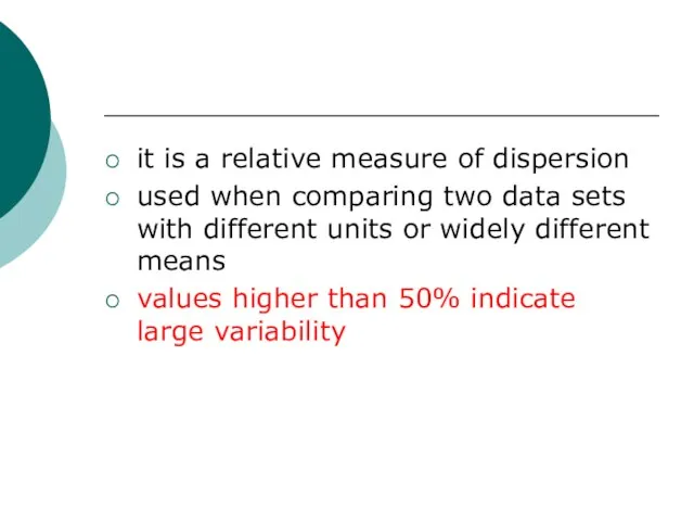
Слайд 33it is a relative measure of dispersion
used when comparing two data sets
it is a relative measure of dispersion
used when comparing two data sets
Слайд 34Example – Personal income (thousands CZK)
Example – Personal income (thousands CZK)
Слайд 35Percentiles (Centiles)
value below which a certain percent of observations fall
scale of percentile
Percentiles (Centiles)
value below which a certain percent of observations fall
scale of percentile
Слайд 36Deciles
divides a distribution into 10 equal parts
there are 9 deciles
D1 – 1st
Deciles
divides a distribution into 10 equal parts
there are 9 deciles
D1 – 1st
Слайд 37divides a distribution into 4 equal parts
Q1 - 25 percent of values
divides a distribution into 4 equal parts
Q1 - 25 percent of values
Слайд 39Graphing Techniques
Слайд 40Constructing graphs – Bar graph
x – axis: labels of categories
y – axis:
Constructing graphs – Bar graph
x – axis: labels of categories
y – axis:
Слайд 41Arranging the graph
nominal variables – we can arrange the categories in any
Arranging the graph
nominal variables – we can arrange the categories in any
Слайд 45Constructing graphs – Pie graph
Pie chart – a circle divided into sectors
Constructing graphs – Pie graph
Pie chart – a circle divided into sectors
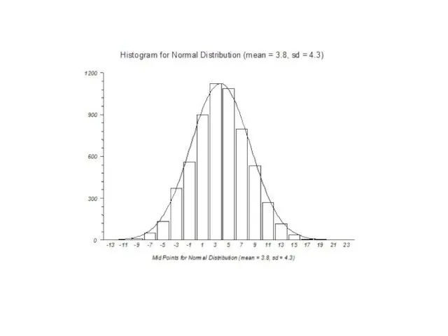
Слайд 47Constructing graphs – Histogram
bar graph for quantitative data
values are grouped into intervals
Constructing graphs – Histogram
bar graph for quantitative data
values are grouped into intervals
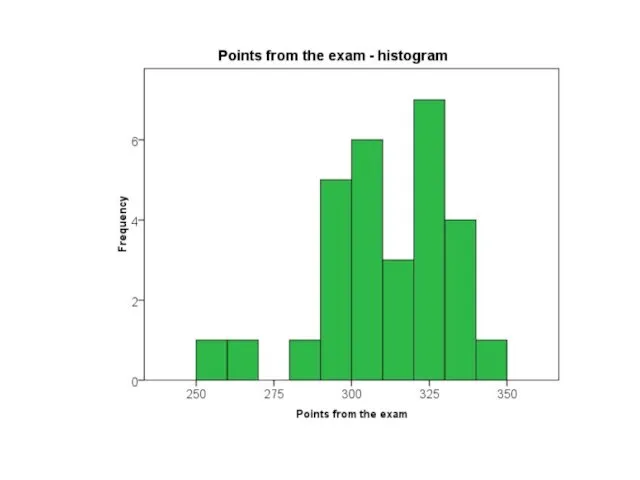
Слайд 49Histogram
Histogram
Слайд 51Constructing graphs – Boxplot
box-and-whisker diagram
five number summary
Constructing graphs – Boxplot
box-and-whisker diagram
five number summary
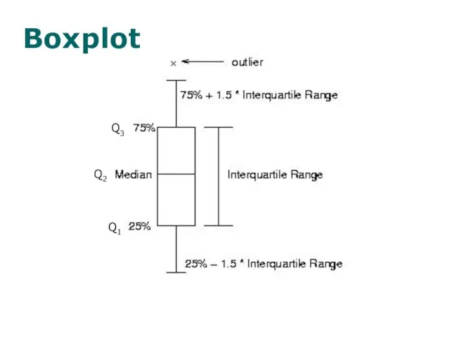
Слайд 52Boxplot
Q3
Q1
Q2
Boxplot
Q3
Q1
Q2
 Сравнение множеств
 Погрешности измерительных приборов. Класс точности
 Задачи на движение в противоположных направлениях
 Деление суммы на число
 Байесовский анализ и сети Байеса
 Презентация на тему Решето Эратосфена
  Многочлен. Основные понятия
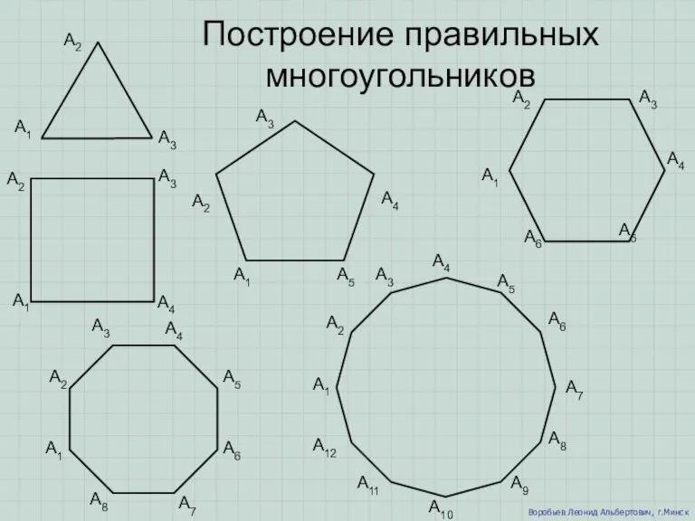 Построение правильных многоугольников
 Решение тригонометрических уравнений. 10 класс
 Доли. 3 класс
 Умножение обыкновенных дробей
 Сокращение дробей. Самоанализ
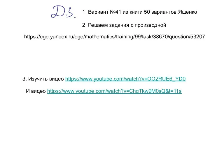 Решение заданий с производной
 Решение задач с помощью пропорций
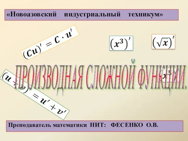 Вычисление производной
 Умножение десятичных дробей
 ES_in_Diag
 Построение сечений многогранников. Построение сечений параллелепипеда
 Тригонометрические уравнения. Арксинус
 Равносильность формул логики. Законы логики
 Одночлены и их свойства. Тест
 Доли. Обыкновенные дроби
 Уравнения и неравенства
 Ломанная линия
 Признаки равенства треугольников. Равнобедренный треугольник
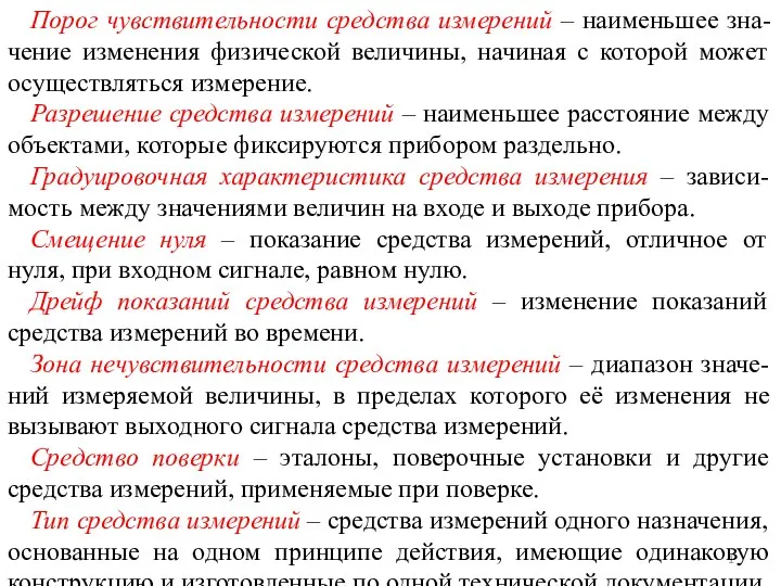 Порог чувствительности средства измерений
 Теория вероятности
 Тренажер по логарифмам